The Front End: Tell Me What Happened AND When It Happened

In life, it seems like you’re always either doing the wrong thing at the right time, or the right thing at the wrong time. So why don’t we take this experience into account when we acquire data or make measurements? After all, it can be a real problem if you only record what happens and not when it happens.
Consider a noisy signal channel. It’s obvious that you run the risk of getting a somewhat “wrong” measurement, as in one that has an error due to the measurement noise. We know we might get the wrong thing, but we usually assume we’ll get it at the right time; i.e., the time we wanted.
But there’s another significant source of noise in a data-acquisition channel. You may not have sampled that signal at the “right” time. And therefore, you might have got the right thing at the wrong time.
Too often, I see measurement systems designed with an obsession on getting the right thing, but with scant attention taken to ensure that it was got (sorry, can’t bring myself to write “gotten,” it’s a Brit thing) at the right time. It’s hard to convince people that “time noise” can sometimes be as much of an issue as “amplitude noise.”
Practically all post-processing of sampled data is predicated on the signal having been uniformly sampled. This crucial element is often mentioned just once, in one of the boring early chapters of the Signal Processing textbook that today’s impatient young engineers are keen to move on from. So, cut this out and stick it inside the front cover of your textbook:
You can’t filter or transform a set of measurements unless you know when they were measured. A data point y(t) is a point on a plane with coordinates (t,y) and you do not have full information about that point and its influence unless you know both t and y.
The obvious way to address this is to time-stamp all your measurements. I had that drilled into me as a young engineer. Every time you measure something, write down the time when you measured it. The result, after a sequence of measurements, is a proper (t,y) dataset. It doesn’t matter too much if you don’t take your readings at constant intervals. There are interpolation techniques that do a good job of reconstructing an underlying implied continuous process (a voltage, a temperature, a carrier frequency, anything really) from data points separated by known irregular intervals.
If the irregularity of the measurement issues is unknown, of course, it’s another matter entirely.
Points of Uncertainty
The killer assumption we make too often is that when we set up some kind of sampling system (for example, using an ADC), we just connect some sort of sampling clock. And hey, presto, we’ll get a dataset of uniformly sampled data points, spaced in time by a known interval. But with any real clock, the frequency is never quite constant, and so the interval between sampling points is also slightly variable.
This isn’t a problem that goes away suddenly when the uncertainty of your measurement timing is reduced below a certain threshold. The clocks used to time the acquisition or reconstruction of signals between analog and digital domains will often suffer from a certain amount of jitter—an inconsistency in the position of the edges of the clock signal. The mean frequency of the clock may be correct, but each edge may be located a small, unknowable distance away from the “ideal” position.
You can think of this uncertainty in edge timing as being the result of phase modulation by some otherwise unknowable signal. Modulation in the time domain has an impact in the frequency domain. Spectral analysis (e.g., taking a fast Fourier transform, or FFT) of an ideal clock’s fundamental component should show up as a single frequency value—a nice sharp line in the FFT. But if the clock’s edges are moving in time, additional sideband frequencies are generated. This smears out the sharp fundamental into a broader spectrum. But why is this a problem in a “digital” system? Why should the frequency spectrum of a clock have any impact on the performance of a system using that clock?
Here’s a concrete example. I wanted to assess the impact of various clock-generation methodologies on audio reproduction as part of a project to build a multichannel interface for PDM microphones. These microphones contain a delta-sigma modulator front end that spits out a one-bit stream clocked with an incoming clock from the interface. That one-bit stream is heavily decimated in the interface to filter off the high-frequency noise inherent in the ADC, leaving nice multibit audio at a more conventional sample rate. Standard stuff.
Here’s the important bit: Anything that modulates the clock, modulates the output data in essentially the same way. If the clock used by the ADC is smeared out in frequency, the data that comes out of the system will inherit that smearing. That’s because when it is reproduced, or analyzed by an FFT, the time information in the wobbly clock edges that caused the smearing will be unavailable; therefore, they can’t be taken into account. Even though we’re talking about clock edges that might be in the wrong place by only a fraction of a nanosecond here and there, the mismatch between where sampling actually happened and where you assume it happened without the a priori information is enough to mess things up in the data.
If this seems a bit remote to you, consider this: Sometimes all of the information in a signal is in the time domain, and none is in the amplitude domain. It has long been known, for example, that much of the information in a complex, bandlimited signal such as speech can be extracted from knowledge only of the positions in time of the zero crossings. In that case, we get a set of data points (t,0) with no amplitude content at all. Yet it’s usually pretty intelligible.
Other examples are binary PDM and PWM—pulse-density modulated and pulse-width modulated—signals. These signals are processed in such a way that the value of the “1” and “0” state voltages don’t contribute to the reconstructed signal. The information is contained in the duty cycle of the binary stream.
Eyeballing It
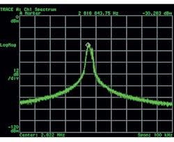
1. The 2.822-MHz (nominal) clock from crystal-referenced FLL.
Let’s go graphical. Figures 1 and 2 show spectral analyses of two versions of a 2.822-MHz clock intended to feed a PDM microphone interface on a Cypress PSoC 6. PDM technology now dominates the consumer audio microphone space. These were captured on a venerable Hewlett-Packard (now Keysight) 89410A, a now-obsolete but much-loved workhorse of my testbench for over 20 years. If you like tight, sharply defined spectral lines, it’s not hard to choose.
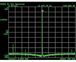
2. The 2.822-MHz (nominal) clock from crystal-referenced PLL.
The clock of Fig. 1 was derived from a fast-starting, low-power frequency-locked loop (FLL), while Fig. 2 shows the spectrum of the system phase-locked loop (PLL). That block takes a little longer to start up and consumes a little more power. Both of them were driven by a reference frequency sourced from the system crystal oscillator, running with my favorite audio crystal frequency of 17.2032 MHz (available from my favorite crystal supplier IQD, as the LFXTAL063075).
Now jump to Figures 3 and 4. For this test, I used the PDM emulation hardware in an Audio Precision APx525. When stimulated by the applied clock, the PDM interface produces a one-bit signal modulated by your choice of test signal, in this case a 1-kHz sinewave at −20 dBFS (okay, call me old-fashioned). The plots show the spectrum from 0.9 to 1.1 kHz; I suspect a little bug in the axis marking routine…
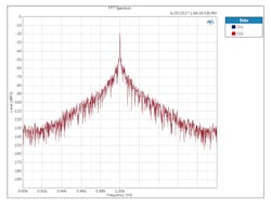
3. Close-up of 1-kHz test PDM tone at −20 dBFS clocked from Figure 1’s clock.
So, no prizes for guessing which plot of the audio result is associated with each plot of the clock’s spectral makeup. Fig. 4 is nice. Fig. 3 would get you kicked out of any audio-savvy company. And there are non-audio measurements requiring this level of cleanliness, too. If you’re looking for closely spaced vibrational modes in stiff structures, you don’t want the ADCs converting your accelerometer signals to be hampered by bad clocks like this. You’ll get this effect with whatever architecture of ADC you use. It’s not just a delta-sigma or one-bit thing.
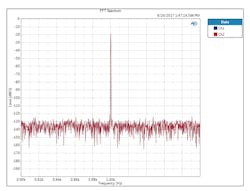
4. Close-up of 1-kHz test PDM tone at −20 dBFS clocked from Figure 2’s clock.
There was never any real danger that we would use the low-quality clock of Fig. 1 in our solution. Not on my watch (maybe in my watch, but that’s a low-power microphone discussion for another day). Rather, I felt it was important to make these measurements, to show the less-experienced and the skeptical amongst my colleagues that, when it comes to audio, you can’t cut corners with clocking.
Have you had a hard-to-find performance problem that turned out to be down to clock spectral quality? Let me know!

About the Author
Kendall Castor-Perry
Senior MTS Architect, Programmable Systems Division
For nearly four decades, Kendall Castor-Perry has been chasing signals through electronic systems, wringing out the information they are hiding. He’s a world-class authority on filters and precision analog circuit engineering and a tireless champion of the needs of the customer. He has been widely published and syndicated, especially when sharing his extensive filtering knowledge as “The Filter Wizard.” He holds a BA in Physics from Oxford and an MBA in MBA stuff from London Business School. Kendall is currently Senior MTS Architect in Cypress Semiconductor’s Programmable Systems Division, pushing on the performance:power:price boundaries constraining tomorrow’s critical sensor-processing systems.
Comment About the Article
To join the conversation, and become an exclusive member of Electronic Design, create an account today!

Leaders relevant to this article: