SPICE It Up: Understanding and Using Op-Amp Macromodels

Download this article in PDF format.
Modeling the performance of an analog device with SPICE is one of the standard techniques used by circuit designers to perform initial characterization and performance analysis before putting together a real-world circuit and testing it on the bench (Fig. 1). SPICE is an acronym for Simulation Program with Integrated Circuit Emphasis. It was originally developed at UC Berkeley in 1973 to verify transistor-level operation of a design before building the integrated-circuit equivalent.

1. TI’s TINA-TI SPICE program helps analog designers solve circuit problems in the virtual world (Source: TI Blog: “SPICE it up: Why I like TINA-TI (part 1)”)
As a tool for the IC designer, the first SPICE programs used detailed mathematical formulas that modeled the behavior of each individual resistor, inductor, transistor, etc. An IC designer requires a high level of accuracy to emulate the expected performance of the final design. As the IC complexity increases, so does the level of processing power needed to run the SPICE simulation.
The design group can use a powerful engineering workstation that runs for several hours to yield a precise result. Circuit designers, though, are more interested in a program that simulates the main performance characteristics of a design so that they can find and fix obvious problems. The program must also produce results in a timely manner running on a typical desktop or laptop.
Sponsored Resources:
- Trust but verify SPICE model accuracy
- SPICEing Op Amp Stability
- What’s the difference between macro models and behavioral models?
SPICE Model Development: Macro and Behavioral Models
Instead of modeling individual transistors, integrated-circuit manufacturers have developed macromodels that simulate most of the performance specifications of an op amp by treating it as a black box that contains mathematical functions representing the internal functions. The SPICE macromodel implementations are simplified groupings of the individual component equations, so the macromodel runs much faster than the design-group simulation and is more robust.
Each analog circuit is different. Thus, designers carefully tune and test each macromodel to ensure that it accurately simulates the behavior of the real device. Nonetheless, subtle differences exist between the performance of the real and modeled devices. The macromodel, for example, may omit second- or third-order effects in the interest of execution speed, or use a piecewise-linear lookup table to represent a smoothly varying curve. As the cost of processing power declines, models are becoming more accurate, and manufacturers are continually refining them.
Another way to simulate device operation is through a behavioral model. This technique models the operation of several components, typically grouped as a functional block, with various SPICE devices. The focus is on the input and output characteristics of the block, so the SPICE model may bear little resemblance to the circuit in the device.
A behavioral model accomplishes its task using relatively few components. This speeds execution time but may omit some of the secondary circuit effects. Most SPICE programs include the capability to define behavioral functional blocks and add them to a macromodel.
Although a simulation can’t replace the real device, an accurate macromodel can help the designer quickly identify many design issues and potentially shorten the design cycle.
A Macromodel Example
What building blocks go into a macromodel? Figure 2 shows a macromodel developed by Texas Instruments to simulate the architecture of its CMOS op amps. Features include the input common-mode range, MOSFET input-stage transfer characteristics, accurate frequency and transient response, slew rate, rail-to-rail output swing, and output short-circuit current.
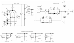
2. A typical op amp macromodel includes both transistor-level and behavioral blocks. (Source: TI Application Report: “AN-856 A SPICE Compatible Macromodel for CMOS Operational Amplifiers” PDF)
The op-amp macromodel is embodied in its SPICE netlist. It’s a text file that describes the interconnections between components—MOSFETs, diodes, inductors, capacitors, resistors, etc.—and standard blocks such as voltage-controlled voltage sources (VCVSs) and voltage-controlled current sources (VCCSs). The SPICE program contains standard mathematical representations of active and passive components and building blocks, letting the user specify the parameters for each one. With MOSFETs, for example, the user can choose between several device models with different levels of complexity.
The CMOS op-amp macromodel contains several stages. The input stage includes several characteristic features: nonlinear input transfer characteristics, offset voltage, input bias currents, second pole, and quiescent power-supply current. Its heart consists of a differential amplifier comprising two simplified MOSFET models. The input offset voltage is modeled with an ideal voltage source (EOS) while input bias and offset currents are modeled by properly setting the leakage currents on the input protection diodes DP1–DP4. Current source I2 and series resistors R8 and R9 model the quiescent current—the current through R8 and R9 increases as the supply voltage increases, effectively modeling the operation of the real device.
R8 and R9 also form a voltage divider that establishes a common-mode voltage VH for the model directly between the rails. VCVS EH measures the voltage across R8 and subtracts an equal voltage from the positive supply rail. The resulting node (98) provides a reference point for many stages in the model. G0, another VCVS, and resistor R0 model the gain of the input stage.
The frequency-shaping stages add multiple poles and zeros to increase accuracy and precisely shape the macromodel’s magnitude and phase response. Each frequency-shaping stage has unity dc gain, making it easier to add poles and zeros without changing the low-frequency gain of the model.
The common-mode gain is modeled with a common-mode zero stage whose gain increases as a function of frequency. This stage consists of G4, L2, and R13. A polynomial equation controls VCCS G4: the circuit sums the voltages at each input pin (nodes 1 and 2) and divides the result by two to simulate the input common-mode voltage. The dc gain of the stage is set to the reciprocal of the amplifier’s common-mode rejection ratio (CMRR). Inductor L2 increases the gain of the stage by 20 dB/decade to model the CMMR roll-off that’s a characteristic of many amplifiers. The common-mode zero stage output (node 16) is fed back to the EOS source to provide an input-referred common-mode error.
The final frequency-shaping stage sends the signal to the output stage. This models several important functions including dominant pole, slew rate limiting, dynamic supply current, short-circuit current limiting, the balance of the open-loop gain, output swing limiting, and output impedance.
The macromodel also simulates rail-to-rail output performance and the dynamic variation of supply current with load. Although the model has many elements, it still executes more than 30 times faster than the individual-transistor model.
“Trust, But Verify” Works for SPICE Models, Too
The phrase “Trust, But Verify” rose to prominence during the 1980s, and was used by President Ronald Reagan many times when discussing relations with the former Soviet Union. The expression is just as applicable to SPICE macromodels: begin by assuming that the model is an accurate representation, but make sure to check its performance against the real device in a few key areas.

3. SPICE models are continually improving, but make sure you understand which datasheet specifications they will accurately reproduce. (Source: TI OPA326 Models)
Start by checking the manufacturer’s netlist and other documentation to make sure that you understand the capabilities and limitations of the model you’ve chosen. Figure 3 shows the comments section of the SPICE model for Texas Instruments’ OPAx320x, a precision, 20-MHz, 0.9-pA, low-noise CMOS op amp with rail-to-rail input and output (RRIO) performance. The model’s applicability is clearly stated.
What are some of the key specifications to check?
Open-loop output impedance ZO is one area where many op-amp models fall short. Proper understanding of ZO over frequency is crucial for the understanding of loop gain, bandwidth, and stability analysis (Fig. 4).
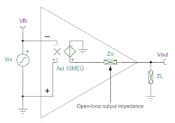
4. An accurate model of output impedance ZO is key to modeling a circuit’s performance and stability. (Source: TI Blog: “’Trust, but verify’ SPICE model accuracy, part 4: open-loop output impedance and small-signal overshoot,” Fig. 1)
Spurred by changes in technology and design innovations such as rail-to-rail output voltages, class-AB bipolar-junction transistor (BJT) output stages have largely given way to rail-to-rail bipolar and common-drain complementary metal-oxide semiconductor (CMOS) designs. Consequently, ZO has changed from the largely resistive behavior of early BJT op amps to a complex impedance with capacitive, resistive, and inductive elements.
ZO appears in the macromodel’s small-signal path between the open-loop gain stage and the output pin. This impedance interacts with the op amp’s open-loop gain Aol, the load, and the feedback components to create the circuit’s overall ac response.
The test circuit in Figure 5 allows you to verify that a model’s ZO matches the data sheet. Inductor L1 provides a short circuit at dc to close the feedback loop while allowing for open-loop ac analysis; capacitor C1 provides an ac short to ground to prevent the inverting node from floating. The ac current source I_TEST back-drives the op-amp output. By measuring the resulting voltage at the output pin, you can determine the output impedance using Ohm’s law.
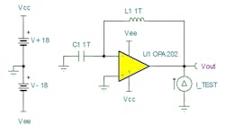
5. The recommended test circuit for output impedance. (Source: TI Blog: “’Trust, but verify’ SPICE model accuracy, part 4: open-loop output impedance and small-signal overshoot,” Fig. 2)
To plot ZO, run an ac transfer function over the desired frequency range and plot the voltage at Vout. Note that many simulators default to showing the results in decibels. If you plot the measurement on a logarithmic scale, Vout is equivalent to ohms.
Figure 6 compares the macromodel ZO to the datasheet for TI’s OPA202, a precision, low-noise bipolar amplifier. The macromodel is a close match. Both impedances are very flat (that is, resistive) up to around 1 MHz, a characteristic typical of classic bipolar amplifier designs.
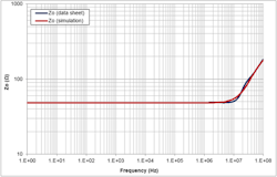
6. The output impedance of the OPA202 macromodel closely matches that of the datasheet (Source: TI Blog: “’Trust, but verify’ SPICE model accuracy, part 4: open-loop output impedance and small-signal overshoot,” Fig. 3)
Of course, output impedance isn’t the only macromodel parameter you might want to verify. There’s an informative series of blogs discussing the testing of other op-amp SPICE parameters: common-mode rejection ratio (CMRR); offset voltage versus common-mode voltage (Vos vs. Vcm); slew rate (SR); open-loop gain (Aol); input offset voltage (Vos); and noise, including voltage noise and current noise.
Practical Applications: Stability Testing
Once we’ve verified the accuracy of the op-amp macromodel, we can use it in a practical application. For op amps, instability in a circuit can manifest itself as continuous oscillation, overshoot, or ringing, and can be very difficult to debug. A good model, combined with the powerful analysis tools available in SPICE programs, can help predict and stabilize op amp performance in the virtual environment before assembling the real circuit.
As an example, let’s use the macromodel for the OPA211, another low-noise precision bipolar op amp.
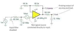
7. Checking the stability of an op-amp circuit often requires changing the “real-world” circuit. (Source: TI Archives: SPICEing Op Amp Stability, Fig. 2)
Checking the response to a small-signal step function or square wave is a quick and easy way to look for possible stability problems. Figure 7 shows the simulation circuit, which differs from the real-world design in several respects. The input filter would slow the input edge of a step function, so it’s disabled. Instead, the input test signal connects directly to the op amp’s non-inverting input.
Similarly, the output circuit of R4 and CL filters the signal Vout seen at the circuit output; Vopamp shows the true op-amp response.
We’re looking for the small-signal step response, so the applied input step is 1 mV. With a circuit gain of 4, this results in a 4-mV step at the output. A large input step would add slewing time and reduce the overshoot.
Figure 8 shows the results of the analysis. In the time domain, the overshoot of Vopamp is 27%. From the graph in TI’s Analog Engineer’s Pocket Reference, this translates into a phase margin of around 38%, below the 45% considered the minimum for a stable circuit. The frequency response indicates amplitude peaking, another tell-tale sign of instability.
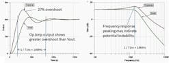
8. The SPICE simulation uncovers problems in both the time and frequency domains. (Source: TI Archives: SPICEing Op Amp Stability, Fig. 3)
Although it’s possible to perform more in-depth SPICE analysis, this simple method is a good indicator of potential stability issues with a simple op-amp circuit. As we’ve discussed, the SPICE simulation is only as good as the op amp’s macromodel, and other components, parasitics in the printed-circuit-board layout, and poor power-supply bypassing can all affect the circuit.
SPICE simulation can provide a high level of confidence in your analog design, but it doesn’t guarantee performance. After identifying and correcting problems during the simulation phase, you should always proceed to build the actual circuit and test it on the bench.
Downloads, References, and Further Reading
Texas Instruments has teamed up with DesignSoft to offer TINA-TI, a SPICE-based simulation program that’s free to download (Fig. 1, again). TINA-TI is suitable for a wide range of analog and switched-mode power-supply (SMPS) circuits and comes preloaded with models for hundreds of TI parts. The program is easy to set up and use, and features powerful dc and transient analysis capabilities, an intuitive graphics-based interface (GUI), and on-screen contextual help.
Several application notes discuss SPICE macromodel development. This helpful application bulletin reviews and compares different op-amp macromodels: AN-856 details the development of a macromodel for CMOS op amps, and AN-840 reviews the current-feedback op-amp topology.
Finally, you can learn more about TINA-TI, read relevant blogs, or post SPICE-related technical questions at the Simulation Models forum of TI’s E2ETM Community.
Sponsored Resources:
About the Author
Paul Pickering
Paul Pickering has over 35 years of engineering and marketing experience, including stints in automotive electronics, precision analog, power semiconductors, flight simulation and robotics. Originally from the North-East of England, he has lived and worked in Europe, the US, and Japan. He has a B.Sc. (Hons) in Physics & Electronics from Royal Holloway College, University of London, and has done graduate work at Tulsa University. In his spare time, he plays and teaches the guitar in the Phoenix, Ariz. area
Comment About the Article
To join the conversation, and become an exclusive member of Electronic Design, create an account today!

Leaders relevant to this article: