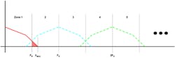
The relationship between a signal’s constituent frequencies and the sampling rate used to quantize them is fundamental. As shown in Figure 1, sampling a signal that has a given spectrum creates a series of images of that spectrum around each multiple of the sampling frequency fS. The baseband signal spectrum is directly copied to bands immediately above each multiple but copied as a mirror image to bands below.

Many aspects of sampling were quantified by Harry Nyquist, who worked on telegraph transmission as well as more general communications theory at Bell Labs. The Nyquist frequency, fN = fS/2, is the maximum frequency component that a sampled signal can have without aliasing. As shown in Figure 1, the frequency bands around multiples of fS are called Nyquist zones and numbered consecutively starting at 1 for the original baseband signal.
The figure also shows what happens when the maximum signal frequency fMAX>fN. If the maximum frequency is too large compared to the sampling rate—or the sampling rate too low for the signal—aliasing occurs. Frequency components above fN corrupt frequencies below it. For example, if fMAX = 1 kHz and fN = 800 Hz, the signal component 200 Hz above fN will corrupt the original signal’s 600-Hz component.
Although most data acquisition applications deal with a baseband signal, communications applications may not. For a thorough discussion of sampling signals in higher Nyquist zones, see “A View of Undersampling” by Hideo Okawara, Verigy Japan, published in EE-Evaluation Engineering, June 2011.
Reducing Aliasing
It makes sense to consider what is meant by fMAX. For a real signal, noise contains frequencies far beyond the intended signal bandwidth. Noise can be reduced by filtering the signal, but higher frequency components will only be attenuated, not eliminated. So, it is necessary to establish a limit to the amount of aliasing that your application can accommodate. Then, you can specify the stopband attenuation that an anti-aliasing filter must provide at fN.
All realizable low-pass filters have three frequency bands: the passband from DC to the -3-dB cutoff, the transition band, and the stopband. The shape of the passband and the width of the transition band are as important as the stopband attenuation. These characteristics cannot be independently or arbitrarily chosen because they directly relate to the nature of your application.
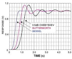
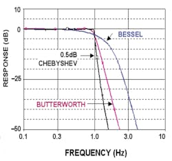
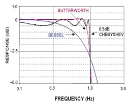
The four parts of Figure 2 show some time- and frequency-domain characteristics for three popular filter types. As shown in Figures 2a and 2b, the Bessel filter gives the best impulse and step responses but has a very gradual -3 dB corner. It’s one of the common filter types used for time-domain work but attenuates higher passband frequencies. For frequency-domain analysis that needed a flatter passband response (Figures 2c and 2d), you probably would select a Butterworth or Chebyshev (type 1) filter, the choice depending on the importance of passband ripple.

Courtesy of Analog Devices
Figures 2a, b, c, and d present details for eight-pole filters. The three types shown are described as having all their zeros at infinity so only their pole locations govern performance. Eventually, all three types will achieve a -48 dB/octave slope in the transition region (8x6dB/octave/pole), but their detailed performance near the -3 dB cutoff is very different.
Bessel and Butterworth Filters
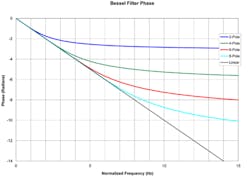
Figures 3a and 3b illustrate the normalized magnitude and phase responses, respectively, for two-, four-, six-, and eight-pole Bessel filters. You would use a Bessel filter if maximally flat group delay were important to your application. These filters have an approximately linear phase response, group delay being the derivative of phase with respect to frequency. This is why the step response has virtually no overshoot: All frequency components are delayed equally.
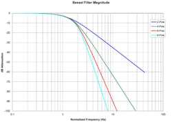
As previously stated, the price you pay for good time-domain performance is poor response in the frequency domain. An eight-pole Bessel filter attenuates signal frequencies two octaves below cutoff by about 0.16 dB. That doesn’t sound like a lot, but as shown in Figure 2d and Figure 4a, an eight-pole Butterworth filter is down only 0.0001 dB, just one octave below cutoff. If the amplitudes of a signal’s frequency components are important to your application, you probably would use a Butterworth filter, not a Bessel.
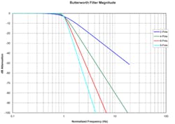
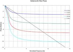
Finally, Figure 4b shows the consequence of the Butterworth filter’s sharp, monotonic, maximally flat magnitude response: nonlinear phase and variable group delay. This is the reason for the large overshoot and subsequent ringing in Figure 2b.
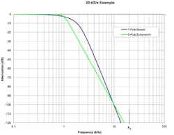
The anti-aliasing performance of either type of filter can be equivalent given a sufficiently wide transition region. Consider an example with the highest signal frequency of 1 kHz and the sampling rate 20 kHz. A large oversampling ratio like this gives more room for a wide transition region as shown in Figure 5. From Figures 3a and 4a, it’s easy to see that a seven-pole Bessel filter can provide 100-dB stopband attenuation at about 10 kHz—the Nyquist frequency for this example. On the other hand, a simpler, cheaper five-pole Butterworth filter also would work. If you need to pass the 1-kHz component with less attenuation, then a higher-order filter is needed with a slightly higher cutoff frequency.
It’s when the oversampling ratio gets very large or very small that filter selection becomes more interesting. Delta-sigma ADCs inherently have an oversampling ratio as large as 64, 128, or more between the input sample rate and the output data rate. An anti-aliasing filter can be very basic and still do a good job because the transition region is so wide.
On the other hand, the digital anti-aliasing filter needed before decimation is very sharp to preserve as much first Nyquist zone bandwidth as possible. If the signal has significant component levels at frequencies higher than the filter cutoff, the time-domain response will be distorted. Of course, the frequency-domain response will be very accurate because these filters are almost perfectly flat to very close to Nyquist. Finally, should all of the signal’s frequency components lie within the passband, the filter’s transition band behavior will have little effect on either the time or frequency domain.
For further anti-aliasing considerations, see “Understanding Noisy Signals,” an August 2005 EE-Evaluation Engineering article on dynamic signal analyzers. In particular, the sidebar accompanying that article discusses a digital filtering technique that eliminates the time-domain step response aberrations caused by a sigma-delta ADC’s very sharp decimation filter.
Sidebar
To Gibbs or Not to Gibbs?
There are many scholarly articles about the Gibbs effect and many more articles that refer to pulse aberrations as being caused by the Gibbs effect. To be sure, there really is a Gibbs effect. It is caused by the failure of the Fourier series to converge uniformly at a signal discontinuity. The speed of convergence depends on the smoothness of the signal, and of course, a discontinuity is hardly smooth.
Nevertheless, few real-life signals have mathematical discontinuities. What actually is happening to cause under- and overshoot as fast waveform edges are processed is not the Gibbs effect. A fast edge has been synthesized in the figure by applying the Fejér kernel to the Fourier series for a squarewave. Fejér was interested in various kinds of convergence and determined that partial sums of the Fourier coefficients did converge uniformly if they were suitably weighted. So, the input waveform in the figure is fast but inherently does not have Gibbs-related under- or overshoot aberrations.
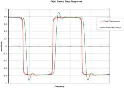
The figure also shows the waveform after passing through a four-pole Butterworth filter. The reasons for the under- and overshoot, the delay, and the slower rise time are the attenuation and phase shifts applied to higher frequency harmonics. In the original waveform, these harmonics serve to smooth out ripples caused by summing lower frequency harmonics and to provide a sharper corner. With the higher harmonics altered by the filter, the output appears to have gained aberrations. Actually, they always were there, just balanced by other harmonics when there was no phase shift or attenuation.
About the Author
Comment About the Article
To join the conversation, and become an exclusive member of Electronic Design, create an account today!

Leaders relevant to this article: