Applying Bayes’ Theorem to clinical trials
Over the years, many writers have implied that statistics can provide almost any result that is convenient at the time. Of course, honest practitioners use statistics in an attempt to quantify the probability that a certain hypothesis is true or false or to better understand what the data actually means.
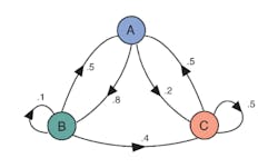
Courtesy of Skye Bender-deMoll
The field of statistics has been developed over more than 200 years by famous mathematicians such as Laplace, Gauss, and Pascal and more recently Markov, Fisher, and Wiener. Pastor Thomas Bayes (1702-1761) appears to have had little influence on mathematics outside of statistics where Bayes’ Theorem has found wide application.
As described in the FDA’s 2010 Guidance… for the Use of Bayesian Statistics in Medical Device Clinical Trials, “Bayesian statistics is an approach for learning from evidence as it accumulates. In clinical trials, traditional (frequentist) statistical methods may use information from previous studies only at the design stage. Then, at the data analysis stage, the information from these studies is considered as a complement to, but not part of, the formal analysis. In contrast, the Bayesian approach uses Bayes’ Theorem to formally combine prior information with current information on a quantity of interest. The Bayesian idea is to consider the prior information and the trial results as part of a continual data stream, in which inferences are being updated each time new data becomes available.”1
Bayes’ Theorem
As explained in the FDA’s Guidance document, prior information about a topic that you wish to investigate in more detail can be combined with new data using Bayes’ Theorem. Symbolically,
p(A|B) = p(B|A) x p(A)/p(B)
where:
p(A|B) = the posterior probability of A occurring given condition B
p(B|A) =the likelihood probability of condition B being true when A occurs
p(A) =the prior probability of outcome A occurring regardless of condition B
p(B) =the evidence probability of condition B being true regardless of outcome A
Reference 2 discusses the application of Bayes’ Theorem to a horse-racing example. In the past, a horse won five out of 12 races, but it had rained heavily before three of the five wins. One race was lost when it had rained. What is the probability that the horse will win the next race if it rains?
We want to know p(winning | it has rained). We know the following:
p(it has rained | winning) = 3/5 = 0.600
p(winning) = 5/12 = 0.417
p(raining before a race) = 4/12 = 0.333
From Bayes Theorem, p(winning | it has rained) = 0.600 x 0.417/0.333 = 0.75. Taking into account the horse’s preference for a wet track significantly changes its odds of winning compared to 0.417 when rain is not considered.2
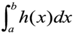
Typically, actual situations are not this simple but instead involve many variables and dependencies. Also, the discrete probabilities of the horse-racing example are replaced by probability density functions (PDFs). Common PDFs, such as the familiar bell curve of the normal distribution, show the likelihood that a variable will have a certain value. Often, researchers need to know that a quantity is larger or smaller than some limit or that it falls within a certain range, which requires integrating part of the area under the PDF curve.
Dr. John Kruschke, Department of Psychological and Brain Sciences, Indiana University, described a learning experiment in which a person is shown single words and combinations of two words on a computer screen. The object is to learn which keys to press in response to seeing a word or combination of words. The lengths of all the response times (RT) between a new word or combination appearing and the correct key being pressed comprise the test data.
All together, there were seven unique words or combinations, called cues, randomly presented to learners often enough that each cue repeated many times. There were 64 learners involved in the study. The objectives were to “…estimate the overall baseline RT, the deflection away from the baseline due to each test item, and the deflection away from the baseline due to each subject.”3
This example is not nearly as large or complex as many medical trials but still was addressed through the Bayesian inference using the Gibbs sampling (BUGS) computer program initially developed by the Medical Research Council Biostatistics Unit in Cambridge, U.K. A great deal of information is contained in the posterior distribution, and Kruschke made it clear that “…the posterior is a joint probability distribution in a high-dimensional parameter space…. [Example PDFs are]… only the marginal distribution[s] of individual parameters, like pressing a flower between the pages of a heavy book. In other words, the posterior specifies the credible combinations of all the parameter values.”3
A joint probability distribution is the probability distribution of a multidimensional vector—each dimension representing a separate variable within a study. In general, the overall PDF cannot be expressed in a closed form and must be integrated using numerical methods.
Analysis
As discussed in Reference 4,“A major limitation towards more widespread implementation of Bayesian approaches is that obtaining the posterior distribution often requires the integration of high-dimensional functions. This can be computationally very difficult, but several approaches short of direct integration have been proposed….”
For many studies, each data point is independent. Here, a data point is the value of a multidimensional vector—the set of answers that a certain respondent gave to a questionnaire. The set of responses given by all the respondents often is considered to be a Markov process, or more particularly a Markov chain because there is a finite number of discrete states that the vector assumes. In a Markov chain, the next value only depends on the current state—neither the preceding states nor their order is important. The successive states observed when repeatedly flipping a coin comprise a Markov chain.
Another concept that is key to addressing practical applications of Bayes’ Theorem is Monte Carlo integration. The Monte Carlo approach can be thought of as a massively parallel set of random trials that is evaluated to estimate a solution. Stanislaw Ulam, who developed the technique when working at Los Alamos in 1946, wrote, “The question was what are the chances that a Canfield solitaire laid out with 52 cards will come out successfully? After spending a lot of time trying to estimate them by pure combinatorial calculations, I wondered whether a more practical method than ‘abstract thinking’ might not be to lay it out say one hundred times and simply observe and count the number of successful plays.”5
Monte Carlo integration approximates an integralRather than flipping a single coin and recording successive outcomes, the Monte Carlo approach to determining that a coin has equal probability of coming up heads or tails is to simultaneously flip thousands of identical coins and then compare the number of resulting heads and tails. A Monte Carlo simulation, on the other hand, would accumulate a very large number of random-value samples from the interval [0,1], assigning heads to values >0.5 and tails to those <0.5. The quantities of each would then be compared to determine bias.
Reference 6 combines the two ideas: “Markov chain Monte Carlo (MCMC) is a collection of sampling methods that is based on following random walks on Markov chains.” Markov chains for which there is a finite probability of transitioning from any state to any other are termed ergodic. The PDF describing the frequency with which the various states of an ergodic chain occur approaches a stationary distribution after a sufficiently large number of transitions—the so-called burn-in time. The transitions from one state to the next form a multidimensional path—a random walk.
Gibbs sampling performs a special kind of random walk in which, “…at each iteration, the value along a randomly selected dimension is updated according to the conditional distribution.” Bayes’ posterior joint probability distribution is defined as the product of conditional distributions, and Gibbs sampling is said to work well in this case.6
Review
The initial design of a medical survey largely influences the usefulness of the results. Bayes’ Theorem allows results from a previous study to be combined with the current study, and it also provides the opportunity to monitor data as the study progresses. However, correctly analyzing the complex joint probability distributions characteristic of this approach requires a statistician trained in the use of Bayes’ Theorem.
As stated in the FDA’s Guidance document, “Different choices of prior information or different choices of model can produce different decisions. As a result, in the regulatory setting, the design of a Bayesian clinical trial involves prespecification of and agreement on both the prior information and the model. Since reaching this agreement is often an iterative process, we recommend you meet with the FDA early to obtain agreement upon the basic aspects of the Bayesian trial design.
“A change in the prior information or the model at a later stage of the trial may imperil the scientific validity of the trial results. For this reason, formal agreement meetings may be appropriate when using a Bayesian approach.”1
References
- Guidance for Industry and FDA Staff: Guidance for the Use of Bayesian Statistics in Medical Device Clinical Trials, FDA, Feb. 5, 2010.
- Boone, K., “Bayesian Statistics for Dummies,” 2010.
- Kruschke, J. K., “Bayesian data analysis,” WIREs Cognitive Science, 2010.
- Walsh, B., “Markov Chain Monte Carlo and Gibbs Sampling,” Lecture notes for EEB 581, April 2004.
- Eckhardt, R., “Stan Ulam, John Von Neumann, and the Monte Carlo Method,” Los Alamos Science Special Issue, 1987.
- Lebanon, G., “Metropolis-Hastings and Gibbs Sampling,” November 2006.
- Skye Bender-deMoll, “Information, Uncertainty, and Meaning,” May 16, 2001.
About the Author
Voice Your Opinion!
To join the conversation, and become an exclusive member of Electronic Design, create an account today!

Leaders relevant to this article:


