
Download this article in PDF format.
Back in May 1995, Bob Pease wrote an article about the “hassler” circuit used by analog great Bob Widlar. The circuit sensed loud voices and would emit a near-ultrasonic squeal to dissuade further yelling or boisterous behavior. Widlar designed the circuit to quiet anyone yelling in his office. It also discouraged typing from a nearby secretary.
The actual circuit Widlar used is lost to history, but Pease postulated his own circuit. Several co-workers agreed that it was close in function to the Widlar circuit. The article is not online, but I found an old bootleg .pdf copy. The schematic was in the inimitable Pease hand-drawn style (Fig. 1). The heart of the circuit is a 22-kHz ultrasonic oscillator with a voltage-controlled frequency. When it senses loud audio at the input, the frequency slows down and drops into the range of hearing, making a nice annoying squealing sound.
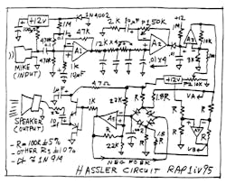
1. Bob Pease designed this “hassler” circuit in 1995. It makes a squealing noise if someone talks too loudly.
As a consultant, I became a stickler for clear readable schematics, so I re-drew Pease’s circuit in my old Cadence OrCAD 9.2 (Fig. 2). I made sure the schematic flowed from left to right and top to bottom. Rather than wrapping it into a U-shape like Pease, I broke mine into two sections with an off-sheet port to connect the two halves. It fits on an A-sized sheet in portrait mode.
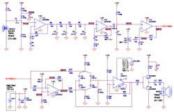
2. The “hassler” circuit redrawn in OrCAD 9.2. CAD makes schematics cleaner and easier to read. The best thing is you can move, rotate, or add components to make things look great.
One benefit of using OrCAD is that you can run Spice simulations on the circuit. Even my old OrCAD 9.2 had decent models for the LMC6484 rail-to-rail op amp and the LM301 uncompensated op amp. Thanks to the diligence of my pals at Texas Instruments, you can get models for their new parts and use those if you prefer. I also have a copy of Altium’s CircuitStudio distributed by Newark.
I’ve heard the old PSpice in OrCAD 9 is pretty superior to most implementations, although LTspice, now part of Analog Devices, is supposed to be very good as well. I know National Instruments’ MultiSim oversees the model creation, making it converge better and have more trustworthiness. I might try this same circuit in those, since the diodes and oscillator in this hassler circuit gives Spice programs a good workout.
CAD schematics show parts with reference designators so we can talk about them. An OrCAD schematic can drive a PCB layout, unlike LTSpice, or all those online Spice tools I consider more hobbyist toys than engineering tools. James C. McLaughlin, my professor at GMI/Kettering, said that it can be easier to understand a schematic reading from the output back to the input. He noted you know what you need at the output, so it is easy to understand things working backward.
Work Back
So, working back from the Radio Shack speaker, Pease used complementary pair Q1 and Q2 to drive the speaker. I guessed the speaker to be at least 32 Ω, since it’s a piezo-transducer tweeter. It’s probably much higher. The output stage is driven by the voltage-controlled oscillator, made from the old LM301A operational amplifier. Pease chose this amp because it’s uncompensated, and that makes it want to oscillate. He left the compensation pins unconnected, but PSpice complains, so I put in a 1-fF capacitor. The circuit will not oscillate naturally in PSpice; the trick is to power the amplifier with a pulse source. That “bang” gets most oscillators started. This is why there are no brown dc bias flags after the oscillator—the bias numbers are not meaningful with that pulse generator as power. The oscillator runs at 18 kHz in my simulation, lower than the 22 kHz Pease intended. I would trust his figures more than Spice.
The oscillator uses a diode bridge as a variable resistor. Its equivalent resistance reacts against C12 to set the frequency. The diode bridge is biased at dc by R16 and R27. They supply 54 µA of current through the bridge, split between the two legs. This puts the diodes on the flatter part of the exponential I-V curve. For small signals, that flatness is like a high-value resistor.
To make that resistance variable, Pease added resistors R18 and R25. When R18 is pulled high, and R25 pulled low, they are in parallel with R16 and R27, respectively. That adds current to the bridge, lowering the effective resistance, since the diodes are now biased further up the I-V curve where the slope is steeper. That lower resistance makes for a higher frequency.
When R18 is pulled low and R25 pulled high, the resistors steal current from the bridge, reducing the diode bias current and increasing the effective resistance. Potentiometer P2 sets the voltage bias of the two resistors. Since you want the oscillator to be fastest with no detected audio, set P2 to bring the resistors to the rails or nearly to the rails. That’s the reason for U1C and U1D—they drive the resistors 180 degrees out of phase. U1D is a simple inverter, so when you set P2 to put the output of U1C at 11 or 12 V, U1D will be at 1 or 0 V. This sets the quiescent frequency of the circuit. U1C also adds gain to the microphone signal.
Ahead of U1C is a diode-capacitor series. Pease called this a rectifier, but it’s more like a high-frequency attenuator. It tends to halve the amplitude of high-frequency signals since the 1M resistor can’t pull the signal up fast enough, before the next negative-going sinusoid comes along. The diode shifts the output of U1B up 0.6 V at dc. At frequency, the capacitor is pulled down instantly by the low impedance of the op amp. When U1B goes high, the diode blocks and the voltage increase on C7 is created solely by R3. U1B has a gain potentiometer that you can twiddle to adjust the sensitivity of the circuit to voices and noise. Capacitor C8 gives the amplifier a gain of one at dc.
U1B is fed by the input amplifier U1A though four single-pole passive filters. The capacitor C9 means U1A will have unity gain at dc; really low frequencies are rolled off. The input ladder biases this amplifier at 2.9 V. Resistor R1 is needed to bias the Radio Shack electret microphone. Capacitor C2 couples the audio output to the input amplifier.
Getting Spice-y
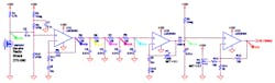
3. The front-end of the “hassler” circuit with dB magnitude probe flags. The flag colors correspond to the plot of Figure 4.
After OrCAD gives us a nice clear schematic, we can use PSpice to figure out the response of the circuit’s filter section (Fig. 3). Doing an ac sweep from 0.1 Hz to 30 kHz shows the bandpass nature of the front end (Fig. 4). The frequency peak is 60 Hz; it’s easier to see if you do a linear plot instead of a log plot. The input amp U1A gives 34-dB gain, while U1B ups that to 50 dB. The final gain stage U1C gives the maximum gain of 65 dB at around 60 Hz.
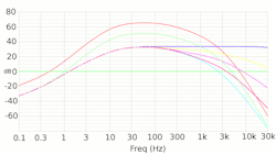
4. The front end of the circuit gives a bandpass response. Colors correspond to probe flags in Figure 3. You can see the five filter traces that have no gain, as well as the final two stages of gain.
Now that you know the optimal frequency, you can do a transient Spice analysis (Fig. 5). I set up an exponential sine-wave source. It increases in amplitude when you set the damping to a negative number. I made the offset 0; the amplitude is 1.5 mV; frequency is 60 Hz; the delay is 10 ms; damping is −15; and I set the phase to 180 degrees, since an initial low-going signal made for a better plot.
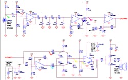
5. The “hassler” schematic with probe flags showing the transient response. Flag colors match the trace colors in Figure 6.
The plot shows P2 biasing the resistor driver amp U1C at 11.2 V (Fig. 6). Inverting amplifier U1D drives its resistor at 0.8 V. I did not want to adjust P2 to push the amplifier outputs to the rails, since amplifiers often use much more current when they hit the rail. That’s fine when delivering a signal, but when there’s no sound, it seemed best to use less quiescent current.
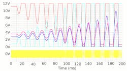
6. The transient response of the “hassler” circuit excited with a 60-Hz rising sinusoid. Colors correspond to the probe flags in Figure 5. I shifted the yellow oscillator output down 2 V so that it does not obscure the other traces.
At 60 Hz, you can see the rate-limiting action of D1, R3, and C7 (Fig. 7). At low amplitudes they just shift the signal upwards by a diode drop. As the amplitude increases, the rising signal can’t keep up, and the amplitude of the signal is attenuated and distorted.
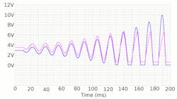
7. The input and output of the rectifier diode. At 60 Hz, the diode level-shifts the waveform up 0.6 V. As amplitude increases, the 1M pull-up resistor cannot slew the capacitor voltage fast enough and the output signal becomes attenuated and distorted. Colors conform to the probe flags in Figure 5.
At 600 Hz, the effect of the attenuation is apparent (Fig. 8). Since the rising signal is controlled by the 1M resistor, the average value of the waveform drops. This would make for some interesting behavior with a real audio signal. I don’t have the patience to learn how to make a stimulus file of an audio signal.
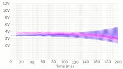
8. At 600 Hz, the rectifier diode output has even more trouble “keeping up.” The signal is attenuated, and the bias level begins to shift with increasing input amplitude. The colors conform to the probe flags in Figure 5.
To make Figure 6 easier to read, I did not measure the output to the speaker. It would have painted over the whole plot in yellow. Instead, I put a differential probe across the input pins of U2. That signal is centered about zero, so I subtracted 2 V from it in the PSpice plot window. That lets us see what’s happening at 0 V for the rest of the circuit.
Zooming in on the transient response of Figure 6 shows the frequency change (Fig. 9). The fast frequency is 18 kHz, and the slow frequency is 3.4 kHz, well into hearing range. Pease said his circuit went from 24 kHz down to 12 kHz. Again, I’ll believe his numbers before a simulation.
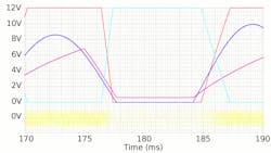
9. Zooming into Figure 6 at 180 ms shows the oscillator slowing from 18 kHz to 3.4 kHz as the audio signal swings the diode-bridge bias resistors from normal to flipped.
Pease said, “Spice lies!” I say, “Spice exasperates.” Any circuit with diodes and oscillators will have convergence problems. I ended up simulating small sections before I got the whole circuit working. For PSpice, I have found setting a small step size helps convergence. It also makes the plots less jagged, at the expense of much longer simulation times. Too small a step creates an error when the output file gets larger than 2 GB. I went down to 10-ns steps and waited forever, before I moved it up to 10 µs. I also lengthened the simulation time from 10 ms to 200 ms, which gave that useful plot in the Figure 6.
If PSpice still won’t converge, I set the transient time point iteration limit to 1000, and check the box, “Use GMIN stepping...”. If it fails to converge on the bias point calculation, I increase both dc bias point iteration limits. I have the “blind” limit at 350, and the “best guess” limit at 350. If the simulation still won’t converge, I loosen up the tolerances. When I had problems, I remember setting RELTOL to 0.005, VNTOL to 5 µV, ABSTOL to 5 pA, CHGTOL to 0.05 pC, and GMIN to 1-19 S (siemens).
You can try more iterations and make things even looser if it still won’t converge. After that, I start adding 1-Ω resistors in series with the diodes. You can also try different amplifiers. I saw little need for the rail-to-rail LMC6484 in this circuit, so I tried it with LMC660 amplifiers. I also used the LMC660 for the oscillator U2 and it seemed to work. After I got small chunks of the circuit converging with those amps, I went back to the LMC6484 and the LM301A, in honor of Pease.
Bob Pease thought Spice made engineers lazy. He feared we would sit and believe simulations instead of going out to the lab and soldering up some wires. Things have changed. The days of DIP (dual inline plastic) packages are fading. Components are surface-mount, not through-hole. Whipping up an “air ball” circuit prototype is rarely practical. I believed it when my high school football coach used to say, “you practice like you play.” I don’t want to prototype in DIP and then have to switch to surface-mount for the production design. Plus, simulations can give important insights.
In the original article, Pease laments that the circuit is sensitive to air-conditioning noise. Well sure, that’s because it’s tuned to 60 Hz. I would think a 1000-Hz bandpass filter would be better at detecting speech and loud noises. Add your ideas and tweaks to the comments. There’s a nice bit of analog in this circuit, even if you just use it as a learning experience.

About the Author

Paul Rako
Creative Director
Paul Rako is a creative director for Rako Studios. After attending GMI (now Kettering University) and the University of Michigan, he worked as an auto engineer in Detroit. He moved to Silicon Valley to start an engineering consulting company. After his share of startups and contract work, he became an apps engineer at National Semiconductor and a marketing maven at Analog Devices and Atmel. He also had a five-year stint at EDN magazine on the analog beat. His interests include politics, philosophy, motorcycles, and making music and videos. He has six Harley Sportsters, a studio full of musical instruments, a complete laboratory, and a video set at Tranquility Base, his home office in Sun City Center Florida.
Comment About the Article
To join the conversation, and become an exclusive member of Electronic Design, create an account today!

Leaders relevant to this article: