A Faster, More Cost-Effective Way to Model High-Performance Motors
Creating accurate 1D models for high-performance motors is challenging because the motors’ performance is affected by nonlinear effects such as variation of flux-linkage with saturation and speed, as well as rotor position and current. These effects are difficult to model, modify, and generalize analytically, especially for highly optimized designs; thus, specialists are needed to build dynamic analytical and multiphysics models.
The conventional approach is fully coupled finite-element-analysis (FEA) co-simulation, but this method costs computational time. Another approach is to tabulate motor performance parameters (flux-linkages as a function of currents, rotor positions and torque/load angles) using FEA.
Multiphysics (2D and 3D) analysis is the most accurate, but also time, computationally, and hardware intensive. Hence, it’s not feasible for “what if” analysis needed to make decisions during product development.1 It also requires different solvers, licenses, and analysts, which complicates the workflow. Low dynamic 1D models (such as analytical models, tables, and response surface models with at least one space dimension2) require less-intensive resources but at the cost of accuracy. Regardless, market demand for a lighter, high-performance electric drive and actuator systems are driving the need for fast and accurate 1D models.
Moreover, growth in automation has led to the integration of electric actuators in human environments. These devices must meet strict standards for safety, noise, vibrations, harshness, and emissions. Satisfying the load requirements, although important, is secondary to the product end-customer. Therefore, system-level analysis is indispensable in the analysis of high-performance electric drives and actuators.
An example of a high-performance drive is an electric-traction system for electric, hybrid, and plug-in hybrid vehicles. It includes an electrical energy source such as a battery, a power converter to process the electrical supply to meet the mechanical load demand, as determined by the controller, and an electric motor to convert electrical to mechanical energy. The motor also can act as an electric generator when the energy flow is reversed.
To overcome multiphysics challenges associated with the simulation of electric drive systems, the entrenched approach is to design the drive components independently. Each physics (electromagnetic, thermal, etc.) is also analyzed independently. The dependency on other subsystems and physics is loosely tied to performance specifications, but it negates component interaction. Integration and system-level performance analysis are done at later stages, which can result in design iterations, driving up costs and increasing time to market.
For example, the power converter and the electric motor can be optimized separately. A converter/electromagnetic optimization will reduce the converter/motor volume and/or mass so as to meet the electrical constraints. However, after system integration, the components may fail to meet other requirements, such as noise, manufacturability, and integration requirements.
In addition, an off-the-shelf optimized solution is only valid for a certain application and may not relate to other applications. This means that high-performance drives should be analyzed as complete solutions, not only at the component level.
To reduce the time to market and costs, a fast and reasonably accurate system-level analysis method is necessary, rather than building multiphysics models. This demand is met by using dynamic 1D models that are suitable for system-level transient analysis and several of orders faster than multiphysics models. Integration and manufacturability should also be included in the analysis.
These models are invaluable in product development for “what-if” analysis during initial analysis, troubleshooting during qualification testing, and design optimization during the detailed design phase.1
Hybrid Method Merges Multiphysics and 1D Analysis
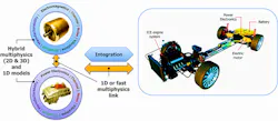
This alternative method combines multiphysics and dynamic 1D models. At the system level, dynamic 1D models are used to set the design criteria and account for subsystem interactions by capturing local transients that may affect the overall system behavior.1 At the subsystem level, the analysis is done using a hybrid of multiphysics (2D and 3D) and 1D models, while the dynamic system-level interaction with the rest of the system is through dynamic 1D or fast multiphysics models (Fig. 1). To further shrink the simulation time, low-penalty assumptions are made, and some multiphysics may be reduced to 1D. Accuracy is improved by experimental calibration.
1. Hybrid multiphysics (2D and 3D) and 1D analysis use 1D models at the system level, while a combination of multiphysics and 1D models are used at the component level. Subsystem interaction is done using 1D models or fast multiphysics models. (motor and converter images courtesy of Oak Ridge National Laboratory)
The software MotorSolve automates 1D model generation for electric motors and generators. Automation lowers the multiphysics knowledge required by the designer. The model export can be reduced order, linear, and nonlinear. The model generation takes into account material nonlinearity, harmonics, geometric dependencies, and approximation of some 3D effects.
These models and, to a larger extent, the nonlinear model have accuracy comparable to FEA, as is illustrated in this article, without the penalty of FEA computation and costs (e.g., co-simulation licenses and analysts). Design information (e.g., stator winding and rotor geometry) isn’t embedded in these models. Consequently, they’re shareable between companies and departments, eliminating the need for non-disclosure agreements.
Steps to Using this Approach
The workflow is elaborated here using a motor similar to that of a BMW i3 electric vehicle. The motor data is courtesy of Oak Ridge National Laboratory (ORNL)3,4 and Jim Hendershot,5 an electric-motor design expert.
Creating the Model
The first step in creating a system-level 1D model using the software is to assign the general settings (Fig. 2). This involves specifying the electrical supply limits (voltage and current), rated speed, global dimensions (outer diameter, length, and clearance between the rotor and stator). The number of poles and slots are entered, and their geometries selected from templates.
2. Motor model after specifying the general setting parameters.
The motor topology can be selected as either interior or exterior rotor with respect to the stator. Model materials are sorted and pre-assigned according to motor parts. If known, the thermal settings (housing, interface gaps, type of cooling, coolant flow-rate, ambient temperature, etc.) and mechanical losses (friction, windage, and stray losses), can be specified.
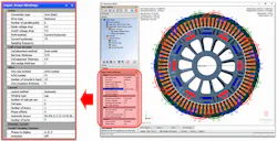
Next, the winding layout is generated automatically (Fig. 3). If desired, it can also be designed manually. The software accounts for coil connections, slot design, conductor sizing, number of parallel paths and strands, and end-windings. You can specify some drive parameters (sine wave or six-step, PWM method, sampling frequency, and device voltage drops, etc.) for a more realistic analysis.
3. Winding design parameters and the automatically generated winding layout.
Performance Analysis
At this stage, the software first automatically builds a model (reduced order, linear, or non-linear), depending on the required accuracy that’s calibrated using FEA. This approach allows for faster analysis compared to traditional FEA.
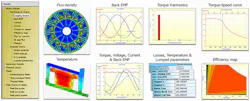
Motor performance analysis (Fig. 4), which includes charts, waveforms, harmonics, and time-averaged analysis charts for power, drive, and motor parameters, are generated with a click. Field distributions (such as flux density, current density, losses, magnet demagnetization prediction, and thermal fields), enable localized hotspots analysis. These virtual experiments are pre-sets provided in the software. Similar charts can be viewed for generator and thermal analysis.
4. Performance analysis using pre-set experiments.
Calibrating and Exporting the Model
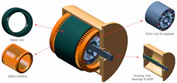
Motors have complex geometries. Figure 5 shows the rotor and stator assemblies, the housing and cooling structures of the BMW i3 motor, and its model. Calibration allows for the simplification of the motor model and physics processes, which saves on simulation time.
5. Calibration allows the simplification of complex geometric models and physics processes, saving computation and solution times while maintaining good-enough accuracy. (Images courtesy of Oak Ridge National Laboratory)
The software has provisions for calibration adjustment factors and flexible analysis methods. Figure 6 shows the improved motor static torque curves after calibrating using the ORNL measured data by adjusting the core stacking and material (BH curve) factors, and switching from a linear to a nonlinear model.
6. Comparison of the model after calibrating the motor static torque using ORNL measured data (left: before calibration, right: after calibration).
After calibrating, or when the model meets the expected performance, we can export it as a response surface model or in VHDL-AMS, Simulink, Opal-RT, and MagNet formats.
Validating the Model
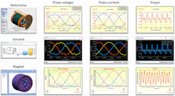
In this example, we exported the model to both Simulink and MagNet to validate the torque at rated conditions (250 Nm, 4800 rpm at 400 A(RMS)). The voltages and currents have the same waveforms and values for the three models (Fig. 7).
7. The validated exported models.
The torques have the same average value but with minor differences in the torque ripple with respect to the MagNet model. In addition, the 1D model used in both MotorSolve and Simulink includes skewing (a 3D effect)—it wasn’t included with MagNet (although it can be taken into account)—to save on solution time. A small time-step was necessary in MagNet to effectively sample the torque ripple. Mesh noise in MagNet may also contribute to torque ripple. Our results confirmed that the exported 1D motor models had the precision of FEA.
Application of 1D Motor Models
Accurate 1D motor models are indispensable in electric-drive systems used in electrified transport, robotic systems, and other servo and variable-speed drives. They’re used to test and verify real-time controllers in software, hardware, and power-in-the-loop (SIL, HIL, and PIL) systems, without the need of a physical machine, or when it’s under prototype. The 1D motor model generates current signals that are converted to power signals using a power amplifier. This is a flexible and cost-effective way of testing electric drives without investing in motors and rotating dynamometers.
The models can also be used to test for compatibility and interchangeability of subsystems at the system level. For example, analyzing the effect of different motors and cooling circuits in a vehicle. Furthermore, they can be utilized in transient analysis, such as startup, response, loading, and faults analysis, with no physical limitations such as power in SIL design and testing for the entire drive. As actuator systems become more electric, ideal dynamic 1D motor models will integrate electromagnetic, thermal, noise, vibration, and structural analysis to meet performance standards.
Conclusion
This automated method allows designers to quickly create more accurate 1D motor models, by significantly reducing the motor analysis workflow. The models can then be used in further system-level analysis with tools such as FloMASTER.
John Wanjiku is the Low-Frequency Electromagnetics Product Specialist in the Mechanical Analysis Division for Mentor Infolytica, a Siemens Business.
References:
1. D. Henninger, A. Zopey, T. Ihde and C. Mehring (2017), “High-Fidelity 1D Dynamic a Model of a Hydraulic Servo Valve Using 3D Computational Fluid Dynamics and Electromagnetic Finite Element Analysis,” International Journal of Mechanical and Mechatronics Engineering, Vol. 11, No. 8, pp. 1476-1482.
2. E. Holzbecher (2012), Environmental Modelling, Berlin Heidelberg: Springer-Verlag.
3. T. Burress (2016), “Benchmarking EV and HEV Technologies” presentation, Oak Ridge National Laboratory (ORNL).
4. B.Ozpineci (2016), Oak Ridge National Laboratory (ORNL) Annual Progress Report for the Electric Drive Technologies.
5. J. Hendershot, http://motorsolver.com/, http://jimhendershot.com/.
About the Author
John Wanjiku
Low-Frequency Electromagnetics Product Specialist, Mechanical Analysis Division
John Wanjiku is the low-frequency electromagnetics product specialist in the Mechanical Analysis Division for Mentor Infolytica, a Siemens Business, Montréal, Canada (formerly Infolytica Corp.). He joined Mentor in December 2016, after his PhD in Electrical and Computer Engineering, majoring in electrical machines. He has over five years of experience in electric machine design and core loss measurements. His areas of interest include the application of FEA in the design of electric devices, electric drives and core losses.
Voice Your Opinion!
To join the conversation, and become an exclusive member of Electronic Design, create an account today!

Leaders relevant to this article:
