New Analog Equals Digital Sleight of Hand
Wrong. One of the major changes that has occurred over the last several years is the development of new display modes variously known as Megazoom™, Digital Phosphor™, Color Accumulate, Analog Persistence™, and TruTrace™. Their capabilities are similar in many ways, but not identical.
Nor is a familiar-sounding name a reliable indication of performance. Tektronix is on the third generation of its DPX technology, and the current Megazoom scope display from Agilent Technologies bears little resemblance to the company’s previous models.
The market for oscilloscopes is very good right now, and there are plenty of uses for distinctive display modes. The growth in high-speed communications continues, semiconductor production is expanding, and the need to transmit local data quickly spawns new buses and networks almost daily.
Fortunately for the designers and test engineers developing these products, today’s ASIC and fast memory device technologies provide the basic scope acquisition performance they require. At first glance, it might not be obvious how significant the new display capabilities also are.
Interparametric Relationships
Oscilloscopes are physical-layer instruments with visual displays. Few if any scopes can tell you whether your data has violated a multibit-, cell-, or frame-based protocol. Most scopes can’t even trigger directly on the occurrence or absence of a specific serial data word, although many claim to be targeted at the communications business. However, they are the best tools available for examining in minute detail the analog artifacts causing a high bit error rate or hair-tearing performance intermittencies.
Wouldn’t life be easier if you could see your signal better? In this case, better involves much more than the display device. Tektronix recognized that acquisition rate was inextricably linked to the amount of information displayed when it introduced InstaVu™ in 1994. Earlier, Fluke/Philips produced a demo board that generated difficult, LF-modulated, real-life waveforms the company claimed only an analog scope could properly display.
InstaVu showed engineers things few had ever seen because it enabled digital acquisition rates as fast as most analog scopes. Repeating successive acquisitions rapidly is important because of the low error rates required in modern data communications. Unless you can capture hundreds of thousands of waveforms/s, for example, you may have to wait a very long time to see a one-in-a-million error. Triggering on the faulty signal usually is not practical because you seldomly initially know what the actual cause of the problem is.
InstaVu operated by overlaying successive short acquisitions to form a 1-bit-deep pixel map. All pixels that corresponded to waveform samples had the same weight regardless of how often they occurred in the constituent waveforms. Every 33 ms when a new map was transferred to the display system, the pixels in that map would be displayed at full intensity. A separate display persistence process altered the color of each pixel through 16 different levels and over a user-selectable period of time. The effect was to present frequently occurring events in the same color, but infrequently occurring events gradually would change color and stand out from the rest.
Although InstaVu dealt with many of the Fluke/Philips waveforms, video engineers emphatically maintained their disdain for DSOs. This group of users relied heavily on the characteristics of traditional analog scopes, and InstaVu did very little for them because it only provided 500-point acquisitions. Not only were video signals dynamically changing, but they also contained tremendous detail. Only a very long memory could capture enough of the signal to be useful.
Even if sufficient data had been captured, the data-compression technology of the day couldn’t display it without losing most of it. Nevertheless, InstaVu highlighted the relationships among acquisition, trigger, and sample rates; re-arm time; memory length; and the display ultimately produced.
Data Compression
The fundamental contradiction that exists between the number of horizontal pixel positions available in a real display device and the much larger number of data points a modern scope acquires had not been resolved. Until the mid 1990s, all digital scopes used the so-called max-min method of data compression shown in Figure 1 (see January 2001 issue of Evaluation Engineering). In this example, 5,000 data points were captured, but not all could be displayed. The finite resolution of the printing process combined with the size of the figure achieves about the same effect as would deliberate compression prior to display.
In max-min compression, the largest and smallest values of each group or frame of 10 points (500 × 10 = 5,000) were displayed at a single horizontal pixel location. In other words, a vertical line was drawn representing the excursion of the signal during those 10 sample intervals.
The analog signal was quantized into a one-dimensional representation, and there was no way to tell anything in detail about what happened during the 10 sample intervals. Similarly, you can see that there is noise at the extremes of the signal in Figure 1, but you can’t tell anything about the nature of the noise from the printed picture.
A less lossy data-compression method was needed. It’s arguable which company first developed a practical version of the intelligent compression algorithm that maps display intensity to the local density of data points. Gould offered TruTrace, Tektronix had the capability in its DPX technology, and LeCroy launched its Analog Persistence feature at about the same time. If you ignore improvements, small variations, and additions, the same basic technique is responsible for the appearance of all compressed-data display modes.
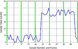
The approach uses display intensity as an additional variable in a low-loss data-compression scheme. Figure 2 (below) is a detailed view of one 50-point section of Figure 1’s 5,000 points, showing the noisy nature of the square-wave signal and five 10-point frames.
Figure 2. Five Successive 10-Point Frames From Figure 1
In Figure 3, separate histograms represent the statistical composition of each of the five frames. The drawing is unusual because the conventional relationship between the horizontal and vertical axes has been reversed. Here, bin numbers run along the vertical axis, corresponding to the range of values of the data points.
The number of times a particular value occurs is indicated on the X axis: in this case, from zero to five for each histogram. The vertical axis corresponds directly to pixel locations, and the horizontal axis is proportional to brightness or color.
The max-min compression example in Figure 3 displays the overall range of signal values that occurred during each frame. The drawing is presented for comparison to the adjacent display of intelligently compressed data, but histograms are not used to produce max-min compression. Finding the maximum and minimum values for a data frame is a simple process.
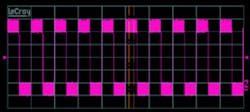
However, in the intelligently compressed example, line segments are plotted with a color or intensity that corresponds to histogram values. For example, it’s easy to see from the resulting display that the noise has several peaks in each frame (because of the higher-valued colors) and that the transition from the top of the square wave to the bottom is fast (because of the zero-value color). Neither of these statements can be made by examining the display of max-min-compressed data. Figure 4 (below) compares complete displays of a signal that has been compressed using the two techniques.
Figure 4. Comparison of Max-Min and Lossless Compression
Although all the enhanced-display scopes use histograms to develop pixel-intensity mapping information, each does so in a proprietary way. Tektronix features its high-speed DPX technology with histogram-based data compression in the new 7000 Series DPOs. Long-record compression is available for up to 1-Mword acquisitions, but the shorter memories associated with very fast trace acquisition rates are provided in a separate accelerated acquisition mode.
In contrast, Agilent designed the 54620 Series Oscilloscopes with data compression as the standard operating mode. Megazoom is the normal display you see, so the scope architecture uses techniques such as ping-ponged acquisition and display memory as well as new 500,000-gate ASICs to simultaneously provide the required scope features and the desired display performance.
A new rendering engine produces up to 25M vectors/s/chan, corresponding to about 4,000 or 5,000 waveforms/s/chan. The 54620 automatically samples at the highest rate and uses the longest memory consistent with the time-base setting. This ensures that the maximum bandwidth can be reconstructed from the sampled data.
As a refinement to the data-compression algorithm, Tektronix modifies the displayed intensity in response to the speed of an edge. Analog scopes don’t display discrete pixels because they draw continuous traces. The closest a DSO can come to a continuous trace is to connect successive sample points with vectors.
In most cases, a display of just the actual sample points can be hard to interpret, and vectors help you to see the signal correctly by connecting the dots. On the other hand, vectors add thousands of pixels to the actual sample points, and in an intensity-modulated display, the intensity of each vector also must be controlled. To mimic the treatment analog scopes provide for waveform edges, vector intensity is related to signal slew rate: the faster the edge speed, the less bright the vector dots.
Displaying the Data
Analog scopes cannot produce aliasing. A DSO’s familiar sampling rate-related aliasing doesn’t occur because there is no sampling process. Spatial aliasing in a DSO also is a quantization artifact, but one caused by the limited number of horizontal pixel locations on digital displays, usually from 500 to 600 in small LCDs. For all practical purposes, analog scope displays are continuous in each axis. To some degree, whether you see the spatial aliasing visual effect as a problem depends on how you look at it.
“The issue is whether the user wants to see the actual data samples or does he want them smoothed and made prettier,” explained Kayle Klingman, principal engineer at Tektronix. “We have measurement data points, and it’s a question of what we do with them.”
Mark Brenner, worldwide business development manager at Tektronix, added, “We know that the customer spends a lot of money trying to capture his signal, and we give him what we believe is the closest thing to reality. We try not to do a lot of massaging of the data.”
Agilent differs from the other manufacturers in the use of a conventional raster-scan, magnetic-deflection, monochrome CRT display. Its obvious advantages are low cost and high brightness. In addition, a 1,000-line raster is generated that provides almost twice the horizontal resolution available on the small LCDs used by other manufacturers. The result is a display with twice the amount of data and less discernable spatial aliasing.
According to Dan Timm, project manager for oscilloscopes at Agilent Technologies, “The capability to increase the horizontal resolution from the 500-point industry norm to about 1,000 points, along with some special data handling, considerably reduces spatial aliasing. Fewer scope-induced artifacts allow users to see real signal aberrations more easily and much sooner.”
A CRT also has an inherent phosphor decay time that serves to integrate successive displayed frames. It’s not just the user’s eyeballs that are integrating intensity variation every 60th of a second. The CRT’s characteristics do improve the comparison between DSO and analog oscilloscope traces. Of course, all your traces are the same green color, and you must rely on trace intensity or blinking to highlight events such as measurements outside of the limits.
In fact, intensity variation in DSOs is nothing new. What is new is the capability to present highly compressed data files as realistic waveforms on a raster-scan display system. A 1984 Gould Model 4040 DSO displayed about 4,000 sample points on a conventional electrostatic-scope CRT. There was no attempt made to modulate intensity to mimic an analog display, but displaying so much data on a small CRT naturally produced intensity variations and added to the display’s realism. Also, because the display system was not raster-based, the intensity of sample-joining vectors inherently tracked their slew rates.
Applications
LeCroy’s analog persistence mode features the capability to measure the parameters of compressed data displays. Like other manufacturers, LeCroy maintains approximately 16- to 21-bit counters to accumulate the number of times each pixel has been hit. Unlike others, LeCroy’s measurements use this detailed pixel activity information and can determine parameters such as the 3-sigma amount of jitter on pulse edges, for example.
These counters have to be large to cope with the wide dynamic range of values produced as thousands of long waveforms are accumulated. Counter size becomes unwieldy, however, because of the very high compression required to map a limited number of intensity levels to the number of pixel hits. LeCroy uses a linear mapping technique but also provides an offset control. The user sets the control to distribute the 16 available levels across those parts of the signal where variations are of interest.
Agilent provides 32 intensity levels and Gould eight. But the comparison among eight, 16, and 32 is not straightforward because of the different compression/mapping methods used and the difference between the appearance of traces on a CRT and an LCD.
Gould’s TruTrace algorithm is implemented by a digital signal processor (DSP) as are many measurement routines in its Classic, Delta, and Ultima Scopes. The acquisition repetition rate in the TruTrace mode is about 10 Hz, but this is more than adequate for the examination of single-shot events often encountered by the company’s industrial customers.
Yokogawa concentrates on maintaining at least a 30-Hz screen update rate for even 1-Mword acquisitions. This is an important capability and emphasizes the interaction between long memory and the acquisition/display update rate when characterizing complex signals such as video. It has accomplished this fast rate through three new data-stream engine ASICs, the graphic control processor being the largest with almost 1-M gates in a 0.35-µm CMOS process.
Similarly, Tektronix, LeCroy, and Agilent have developed their own high-speed data capture/display ASICs. Commenting on the current capabilities of the Tektronix DPX technology, Mr. Brenner said, “We expect there will be more implementations of this technology and that it will be more fully integrated in each successive generation. One of the limitations is the size of the device you can integrate onto a chip. How many transistors can you put in there, and how much heat can you remove?”
Conclusion
As the display characteristics of DSOs approach those of analog scopes, the technical barriers to market entry continue to escalate. Scope market segmentation traditionally has occurred according to guidelines such as bandwidth, sampling rate, memory length, price, and number of channels. But now manufacturers have added displayed information density as another axis of differentiation.
You must determine which scope benefits are most important to you. DSOs are related to analog oscilloscopes, but they’re not at all the same thing. As signal frequencies continue to increase and the DSO becomes your only practical measuring implement, is oscilloscope still the best descriptive term for this kind of instrument?
Would a different name be more useful if it highlighted the mix of a special-purpose computer, acquisition capabilities, and a display device that comprises modern DSOs? After all, the displayed waveform on a DSO is the product of extensive manipulation compared with the very simple and direct signal path from the input to the CRT in an analog scope.
One question that may help decide whether the term oscilloscope remains apt is to ask if you’re looking at waveforms or data. Ms. Klingman from Tektronix described a scope display as a faithfully reproduced collection of data points. Mr. Timm from Agilent was much more concerned about the direct relationship between the appearance of his company’s DSO displays and the waveforms people were accustomed to seeing on a conventional analog scope.
This question also can be approached by asking about the different impressions users have of color-graded and intensity-modulated displays. Dr. Mike Lauterbach, director of product management at LeCroy, said, “Most people prefer color grading, with a minority opting for intensity grading. I think it comes from the way people train their eyes to assimilate information. Certainly, if anyone has used an analog oscilloscope, they’ve trained themselves to use trace brightness as an indication of where the signal is more defined, being less bright where the signal is less defined.”
Tektronix had color grading in its communications signal analyzers, and people in that industry seemed comfortable looking at and interpreting those displays, according to Mr. Brenner. “But, when we introduced the first DPOs, we found that people who hadn’t been in the communications industry would use the intensity-graded monochrome display because it looked more like an analog scope, especially the video people. Recently, we’ve noticed that more digital engineers are making the transition to color graded,” he said, “but we’re not sure whether the video engineers have.”
The question, no doubt, will be answered over time as display devices and ASIC technology continue to improve. It’s a matter of deciding what is good enough. Few DSO users would disagree that if DSO display resolution increased by a factor of 10 in each axis, that the display quality would be equal to that of an analog scope. What about a factor of 5?
Soon, computer displays will achieve resolution increases of ×2 or ×3, and as scopes continue to adopt these displays, they will provide better-looking traces. Think about how an information-rich trace display would help you solve those really difficult signal-related problems. Better yet, get a demo and see for yourself how useful new scope display modes really are.
Acknowledgements
The following companies provided information for this article:
| Agilent Technologies | 800-452-4844 |
| Gould Instrument Systems | 216-328-7000 |
| LeCroy | 914-425-2000 |
| Tektronix | 800-835-9433 |
| Yokogawa Corp. of America | 770-254-0400 |
Published by EE-Evaluation Engineering
All contents © 2001 Nelson Publishing Inc.
No reprint, distribution, or reuse in any medium is permitted
without the express written consent of the publisher.
January 2001
About the Author
Comment About the Article
To join the conversation, and become an exclusive member of Electronic Design, create an account today!

Leaders relevant to this article: