Visualizing Field Perturbations With 3-D EM Software

Powerful PCs mean many companies now find it feasible to use 3-D electromagnetic (EM) software to evaluate the effect of internally generated RF fields propagating inside product enclosures. Meantime, when it comes to assessing the product�s immunity to external fields, test engineers operate blindly when conducting an RF immunity test and often are at a loss to explain extraordinary test-system behavior. Could 3-D EM software be used to gain insight on the likely test-field changes caused by the presence of equipment under test (EUT)?
Present Scenario
It is universally accepted that the field inside a test chamber changes when the EUT is introduced. Also, diffraction, reflection, and resonance effects may cause significant perturbation of the field inside the test chamber.
Field distortion within the test chamber may seem unimportant. However, knowledge of the likely direction and strength of re-radiation lobes and the circumstances under which they can occur could prove very useful if you consider that:
� Military RF immunity tests use a field probe inside the test chamber to monitor and level the strength of the test field. � Commercial test chambers have fully reflective floors. � All chambers have weak areas often at the wall edges.Software Description
The feasibility exercise was conducted using the SINGULA 3-D high-frequency simulation program from Integrated Engineering Software. This program uses several numerical techniques such as the boundary element method (BEM), physical optics, and the finite element method.
With BEM, all boundary surfaces are divided into small triangular segments. Field continuity is forced across the boundary, and then the numerical process is used to find the surface integration of the segments. Finally, vector calculus completes the computation to solve for the unknowns. Near and far field data can be presented in a wide variety of 2-D and 3-D formats.
Particularly useful for the purposes of this exercise is the provision of an incident plane wave excitation source. Also, the data is gathered nonobtrusively so there is no risk of a field probe changing the field it is measuring.Using the Software
There are six main steps to obtaining and evaluating the field information:
Geometry
The geometry chosen for the test piece was a simple box with six perfectly conducting surfaces. The box size approximated a standard 19-inch, 4U-high enclosure, a fairly common size. Wavelengths are measured in meters, so the dimensions were converted and rounded up to the nearest whole centimeter. This resulted in dimensions of 50 cm wide and 18 cm high. An arbitrary depth of 50 cm was chosen.
The box can be drawn as 12 individual line segments, following which each face is defined, and finally the interior space is defined as a volume. Alternatively, one face can be constructed in 2-D or 3-D and the box completed by sweeping the face in the appropriate direction.
Sweeping an area proves to be a great timesaver since the generated faces and the volume are defined as part of the sweep process. As an aid to the drawing process, a comments box lists all previous commands and automatically provides updates on the number of points, line segments, surfaces, and volumes.For symmetry, the front face of the box was placed in the Z = 0 plane and centered at the origin (0, 0, 0). The six surfaces were designated as perfect conductors of zero thickness. The volume was not allocated a material. A screen-shot of the completed model is shown in Figure 1a.

a. Eight Points, 12 Line Segments, Six Surfaces, One Volume
b. 1-MHz Field Plot Along Z-Axis (0, 0, 150) to (0, 0, -150)
c. 1-MHz Radiation Pattern
|
Figure 1. Model Screenshot and Initial Test Results |
Assigning Surface Triangular Segments
Numerical solutions are computationally power hungry, and the time to solve them can increase exponentially if care is not taken with the number of segments assigned. If the automatic segment allocation option is chosen, the user is prompted for the approximate total number.
However, the number of segments assigned is very dependent upon the test frequency since a key rule of thumb applied by the software is 10 segments per wavelength, which can be changed by the user. With higher frequencies and large surface areas, the total number of segments can get out of hand, resulting in a processing time of many hours.
The threshold of pain for this particular exercise was set at 15 minutes per solution. Only in those cases where the results seemed suspect were the number of segments increased and the solution rerun.Incident Test Field
The intention was to illuminate the Z = 0 plane with a plane wave of fixed field strength. Consequently, the excitation source selected was a vertically polarized incident plane wave with a field strength of 1 V/m and a direction of travel along the Z-axis from positive Z to negative Z.
Computation
Once the software has the model and the excitation source, the data is calculated at the chosen test frequency. Other test frequencies require the solver to be run again. At up to 15 minutes per run, it pays to plan ahead and have other tasks at hand to make the best use of your time.
Data Display
Once the solution is completed, the software can present the data in a host of ways. The display types include E or H fields, surface currents, and radiation patterns. You can choose to observe data at one point in space, along a line in space, across a plane or surface, or in the form of 2-D or 3-D radiation patterns.
Our interest lies in the field surrounding the EUT. But be mindful of the old adage of garbage in = garbage out. Cross-checks on the validity of the data were made by plotting the E field along a line passing through the center of the model along with the required 3-D radiation pattern.
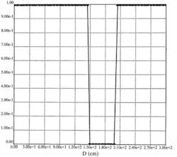
Figures 1b and 1c show the results for the first test frequency of 1 MHz. Figure 1b is the magnitude of the E field passing along the Z-axis from Z = +150 cm to Z = -150 cm. The field level along the line is 1 V/m up to the front face of the box. The field level then drops to zero inside the box.
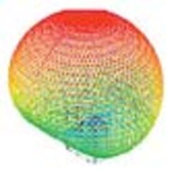
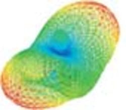
Lastly, the field along the line returns to 1 V/m beyond the back panel of the box. The displayed data is the result of the incident test field and any changes caused by the presence of the EUT.Figure 1c shows the radiation pattern caused by the presence of the box. The maximum value of the lobe (red) is 5 �V/m. Blue is the lowest value on the scale and close to zero. The displayed data for the radiated pattern ignores the presence of the test field.
The plots for all the test frequencies are shown in Figure 2. Note that the vertical axis on the 2-D plots was left on automatic so the maximum value on the vertical axis changes with the maximum value of the measured field.
F = 1 MHz ? = 33 m D = 0.015 ?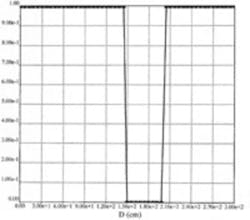
? = 2 m
D = 0.25 ?
SW Max 1.08 V/m
SW Min 950 mV/m
VSWR 1.13:1
Delta Peaks 108 cm
SW Max 1.14 V/m
SW Min 920 mV/m
VSWR 1.24:1
Delta Peaks 54 cm
SW Max 1.48 V/m
SW Min 740 mV/m
VSWR 2:1
Delta Peaks 30 cm
SW Max 1.83 V/m
SW Min 680 mV/m
VSWR 2.69:1
Delta Peaks 15 cm
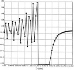
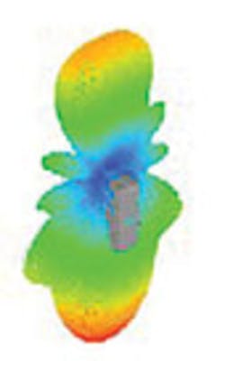
Figure 2. Data Plots
80-MHz Plots
The field along the line starts at 1 V/m and falls gradually to 900 mV/m at 30 cm ahead of the front panel. Then the field drops more rapidly to zero at the front face. The field at the rear of the box mimics the front field but in reverse order. The lobe emanating from the front panel is 29 mV/m maximum.
300-MHz Plots
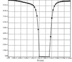
There are field highs at approximately 36, 90, and 144 cm from the front panel. Lows occur at approximately 66 and 120 cm from the front panel. Both the highs and the lows are converging to1 V/m as the distance from the front panel increases.
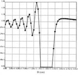
500-MHz Plots
Field highs occur at 18, 48, 78, 108, and 138 cm from the front panel. There are lows at 36, 66, 96, and 126 cm. The field behind the rear panel peaks slightly to 1.1 V/m at 40 cm behind the rear panel.
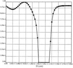
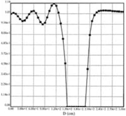
1,000-MHz Plots
Field highs occur 18 cm and 12 cm apart, lows also 18 and 12 cm apart. Over the same total distance, there are twice as many peaks as in the case of 500 MHz. The inconsistency in the distances is due to lack of enough segments.
Interpretation of Plots
The plots in the third column of Figure 2 show that the Faraday cage principle of a zero field inside the box is alive and well in all cases. Before attempting to interpret other aspects of the plots, we should revisit the effects of various EM wave phenomena.
Data plots can indicate the occurrence of various phenomena that happen when an obstacle is put in the path of an EM wave. There are three main cases to look for:
� Diffraction�evidenced by the incident field changing direction such as bending and filling the shadow behind the box. The effect should be most noticeable when the box size is similar to or greater than the test-field wavelength.
� EUT Resonance�evidenced by the EUT re-radiating efficiently. This effect should be noticeable when the EUT dimension approaches a quarter of the test-field wavelength.
� Reflection�when some or all of the incident plane wave is reflected back toward the source and evidenced by the existence of a standing wave. The standing wave is the result of the forward and reflected waves combining as they pass through each other.
The greater the amount of reflection, the higher the peaks and the lower the nulls. The greater the difference between the maximum field and the minimum field, the greater the voltage standing wave ratio (VSWR).
The name standing comes from the fact that there is no forward or reverse motion of the wave. Voltage peaks occur every half wavelength and voltage nulls at quarter wavelength distances either side of the peaks. At the position of the voltage peaks, the amplitude cycles in continuous fashion through positive maximum, zero, negative maximum, zero, and back to positive maximum. When one peak is at positive maximum, the peak half a wavelength away is at negative maximum.
Before proceeding, we should address a widely held misconception. The majority of engineers were introduced to standing waves when attending an educational course on EM wave propagation. The most common experiment demonstrating the existence of standing waves uses a slotted line, which is a length of waveguide with a slot cut along its length and a sliding probe fitted with a detector diode.
RF is fed in one end of the waveguide, and a short circuit is placed on the other end so that a standing wave is formed in the waveguide. The probe is moved along the slotted line, allowing the fixed positions of the nulls to be identified. As the probe slides away from a null position, the voltage can be seen increasing to a peak before decreasing to zero again at the next null.Some young engineers had the impression that voltages of only one polarity existed and that the measured voltages at a point were constant and unchanging. This is a misconception for the following reasons:
� The diode rectifies so it can only detect peaks of one polarity.
� The finite time constant of the detection circuit gives the impression that the voltage measured at a point between the nulls is unchanging when it really is oscillating rapidly.
Getting back to the interpretation of the plots, at 10 MHz, the interaction between the test field and the EUT is almost nonexistent with the field in the chamber acting as if the EUT was not there at all.
At 80 MHz, the dimensions of the EUT are approximately one-eighth of a wavelength, and the test field is showing signs that the EUT is there. The slow reduction in the field strength between 150 and 30 cm from the front face could be due to a small amount of the incident wave being reflected from the front panel. The field taking 70 cm to reach full strength from zero at the rear panel may be evidence of shadowing close to the rear panel.
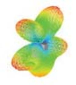
At 150 MHz, the EUT dimensions are a quarter wavelength, and we would expect the EUT to be a good re-radiator if the incident wave couples energy into the EUT. However, with a peak value of only 70 mV/m, the radiation pattern plot shows no evidence of this. The distance between the high and the low points is consistent with the formation of a standing wave, which could mean that the amount of incident power reflected has increased.At 300 MHz, a standing wave has begun to form although the convergence of the highs and lows toward 1 V/m cannot readily be explained. The lobe maximum has doubled with frequency from 70 mV/m at 150 MHz to 140 mV/m at 300 MHz.
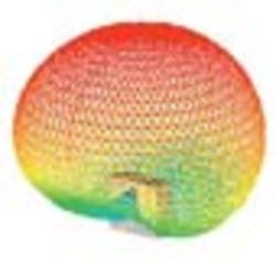
The lobes, though only re-radiating 14% of the incident power, now are pointing up and down. In a semi-anechoic chamber, the wave radiated downward will be fully reflected by the floor. A field probe positioned above the EUT will likely give erroneous readings.
At 500 MHz, the wavelength of the test field is approaching the dimensions of the EUT. The standing wave is even more prominent, which means the amount of the incident wave reflected has increased further. The convergence toward 1 V/m still is very much in evidence.
At 1,000 MHz, the increase in the VSWR indicates that even more of the incident power is being reflected from the front face. The convergence to 1 V/m still is evident and inexplicable.
The slow climb to 1 V/m at the rear of the EUT could possibly be explained by diffraction effects. At 42% of the incident field strength, the forward pointing lobe could result in mutual coupling between the EUT and an antenna. The rear-pointing lobe would be absorbed by the back wall cladding. At almost a quarter of the incident field strength, a field probe caught in one of the side lobes will likely give erroneous readings.Conclusion
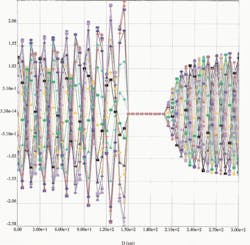
The existence of a standing wave was confirmed using the software�s time-angle capability. This allows snapshots to be taken of the field around the EUT. A particular angle, say 10�, is selected and the instantaneous waveform plotted. A second snapshot then is taken for 20� and so on. By playing the plots in a loop cycle such as Windows Media Player, the action of the wave can be observed in time.
For the 1,000-MHz test field, plots of the instantaneous field along the line 0, 0, 150 to 0, 0, -150 were taken at 20� intervals and plotted on the same sheet of paper. A print version of this process is shown in Figure 3.
The convergence of the standing wave to 1 V/m can only be explained by the amplitude of the reflected wave being attenuated severely with distance. The medium the wave is propagating through has no loss associated with it, and the incident wave propagates through it without loss. So there is no obvious reason for the change in �amplitude.
Obviously, the conditions in a real test chamber are quite different from the ideal conditions described in this article. The incident test field is not a plane wave, and a reflective floor adds considerable uncertainty regarding field perturbations. However, once out of the question on cost and time grounds, 3-D EM software now can be used in a novel way to help provide better visualization of the wave dynamics in the test arena as well as the design arena.
FOR MORE INFORMATION
on SINGULA 3-D Software
April 2006
About the Author
Comment About the Article
To join the conversation, and become an exclusive member of Electronic Design, create an account today!

Leaders relevant to this article: