New Position Sensors Follow Many Paths to Precision

By the start of the 21st Century, the classic limit switch had been largely replaced by the hall-effect sensor, but both were handicapped by their binary outputs. System designers seeking to control the positions of mechanical devices had only one bit of data to work with—not optimum for control loops. The last several years, extending into 2015, have seen remarkable innovation in position-sensing technology, both in terms of resolution (now surpassing 28 bits of precision) and in relative immunity to stray fields. (For a list of older technologies that were developed to supplant the mechanical micro-switch, see the sidebar, “Older Distance-Sensing Technologies”.)
Texas Instruments’ 2- and 4-Channel-Inductance-to-Digital Sensors
In late 2013, Texas Instruments introduced its single-channel LDC1000, a unique position sensing semiconductor device with 20-bit precision based on a technology that can be described as an “inductance-to-digital converter.” This April, TI introduced a multi-channel version, the two-member LDC1614 family, which provides either two or four matched channels and up to 28-bit resolution—all in a single integrated circuit.
Anyone familiar with the electronic musical instrument called the Theremin will grasp the concept, although not necessarily the engineering, that goes into translating that concept into a digital-output measuring device with 28-bit precision. (To be precise, there are two sensors in in a Theremin: one for the pitch of the output sine wave, the other for volume control.)

In any channel of a TI LDC device, what is being digitized are the de-tuning effects of nearby conductors on LC tank circuits (Fig. 1). Typically, the tank coil is a small helix in a PC board. In parallel with the coil is a fixed capacitor. The tank resonant frequency on the latest devices can be anywhere from 1 kHz to 10 MHz. (On the original single-channel LDCs, the range was 5 kHz to 5 MHz.)
This file type includes high resolution graphics and schematics when applicable.
In operation, the tank circuit is driven at its resonant frequency. Some of the radiated energy can be picked up by a nearby conductor, and eddy currents in that conductor will generate a field that creates opposing currents in the tank coil. An ac current in a coil will generate a field that causes eddy currents in nearby conductors. The eddy currents depend on the distance, size, and composition of the target conductor. In turn, the eddy currents then generate their own field, which opposes the field around the coil.
What the TI LDC devices measure is an equivalent parallel resonance impedance, Rp, which is related the distance, d, to the external conductor, where:
Rp(d) = (1/([Rs + R(d)]) × ([Ls + L(d)])/C
The d designation indicates that those variables are functions of the distance to the disturbing conductor.
Meanwhile, there’s a lot going on inside the LDC. It measures the impedance and resonant frequency of the tank and uses that information to regulate the oscillation amplitude to a constant level while monitoring the energy dissipated by the resonator. It simultaneously solves for Rp. Rp and frequency are output as digital values via the I2C interface. For more information about applications for these devices and some background about the history of this technology, see “Redefining Inductive Sensing” at electronicdesign.com.
Late last year, Analog Devices announced its ADXRS290, a high-performance MEMS pitch and roll (dual-axis, in-plane) angular rate sensor gyroscope ideal for such applications as optical image stabilization, platform stabilization, and wearable products. It’s based on a resonating disk sensor structure that enables angular rate measurement about the three axes normal to the sides of the package. Angular rate data is formatted as 16-bit twos complement and is accessible through a SPI digital interface. The device incorporates programmable high-pass and low- pass filters that allow it to achieve a noise floor of 0.004% per root Hz. Its sensitivity spec is 200 LSBs per degree per second.
The data sheet uses explains the operating concepts fairly succinctly (Fig 2.)
Essentially, the MEMS device operates as a vibratory rate gyroscope to sense pitch and roll displacements and report their angular displacement rates. There are four coupled structures like the one shown in the figure, all fabricated in polysilicon. Each structure comprises an electrostatically driven resonating disk that produces the necessary rotating velocity element needed to generate a Coriolis torque when experiencing angular displacement.
After demodulation and analog-to-digital conversion, the rate signal is filtered using a single-pole band-pass filter. The high- pass and low-pass poles of this filter are programmable via the digital interface.
The gyro runs off 5 V, but the sensing structure requires 31 V, so the gyro incorporates a step-up dc/dc converter. This requires an external 1-μF capacitor, which does require some board space in the final design. The MEMS itself comes in a 4.5 × 5.8 × 1.2 mm, 18-terminal cavity laminate package. Output is via a 4-wire SPI bus.
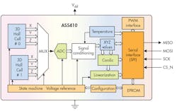
ams’ Dual-Pixel AS54xx Family
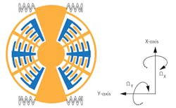
Earlier this year, Electronic Design reported on a new generation of 3D magnetic position sensors that can sense magnetic flux in three dimensions, permitting their use in a wider range of position sensing applications (see “Overcome Stray Field Interference in Magnetic Position-Sensor ICs”). Known as “3D dual-pixel sensor ICs,” they help machine designers comply with the new functional safety standards developed for vehicles with multiple magnetic-field-inducing electrical systems. The technology was developed by ams, an Austrian sensor maker.
The usual approach to protecting hall-effect sensors from stray fields is to shield them. This is often unsatisfactory for a number of reasons, cited in the article above.
What is usually done is to place the position sensor very close to a magnet that has very high remanence (Br). This improves the signal-to-stray-field ratio and, in fact, the overall SNR. Unfortunately, really strong magnets made out of materials such as NdFeB are as much as 10 times more expensive than cheap hard ferrite or plastic-bounded magnets. The approach that the ams engineers came up with – and made work – is a dual-pixel magnetic sensing element (Fig. 3). Using two pixel cells instead of one makes it possible to apply differential measurement techniques, because each pixel cell can measure all three vectors of the magnetic field: Bx, By and Bz. In ams’ AS54xx sensor family, the two pixel cells need to be separated by 2.5 mm.
The original Electronic Design article includes an illustration of the mathematics. Essentially, it shows that when the magnet is exactly centered over the package of the IC, the north-to-south pole transition of the magnet is exactly between the two pixels. Since the pixels are 2.5 mm apart, there is a ±1.25 mm phase shift between the responses for the two pixels, from which the algorithm in the sensor’s internal processor can derive two differential signals, representing x and z vectors.
If a stray field is present, it probably comes from a source much further away from the sensor than the field from the paired magnet is. It has the identical effect on both pixels. This is what enables the differential of position measurement. The longer explanation in the original argument is more rigorous, but that’s the gist of the explanation. In brief, the position of the sensor magnet can be extracted through an arctangent calculation.
AS54xx Characteristics
ams’s AS54xx series of automotive-qualified position sensors provide 14-bit resolution. They are usable between -40°C and 150°C, with no external temperature compensation. Data sheets cite an input range from 5 to 100 mTesla. Other features include integrated self-monitoring, a safety layer that provides protection in the event of a failed ground connection or power supply, as well as under- and over-voltage protection. An EEPROM self-check detects bit-flips.
The dual-pixel differential principle of operation doesn’t just provide for stray field immunity; it also eliminates the need to offset for drift over temperature and time.
This file type includes high resolution graphics and schematics when applicable.
About the Author

Don Tuite
Don Tuite (retired) writes about Analog and Power issues for Electronic Design’s magazine and website. He has a BSEE and an M.S in Technical Communication, and has worked for companies in aerospace, broadcasting, test equipment, semiconductors, publishing, and media relations, focusing on developing insights that link technology, business, and communications. Don is also a ham radio operator (NR7X), private pilot, and motorcycle rider, and he’s not half bad on the 5-string banjo.
Comment About the Article
To join the conversation, and become an exclusive member of Electronic Design, create an account today!

Leaders relevant to this article: