How to Design a Good Vibration Sensor Enclosure (Part 1)

This article is part of the Analog series: How to Design a Good Vibration Sensor Enclosure

Members can download this article in PDF format.

What you'll learn:

What is modal analysis?
Evaluating vibration sensor enclosures and their natural frequencies.
Determining the most important modes and frequencies with the mode participation factor.
A close look at the Timoshenko equation for vibration.

A well-constructed mechanical enclosure design for a MEMS accelerometer will ensure that high-quality vibration data for condition-based monitoring (CbM) is extracted from the monitored asset. The mechanical enclosure used to house a MEMS accelerometer needs to have a frequency response better than the integrated MEMS.

This article uses modal analysis to deliver the natural frequencies possible with enclosure designs. Guidance on vibration sensor design is provided using theoretical and Ansys modal simulation examples. It’s shown that geometry effects, such as enclosure shape (e.g., a cylinder or a rectangle) and height, dominate the natural frequencies in enclosure design.

Mechanical design examples are provided for housing single-axis and triaxial MEMS accelerometers with 21-kHz resonant frequency. This article series also offers guidance on epoxy integration in enclosures, as well as cable installation and mounting options for sensors.

What is Modal Analysis and Why is it Important?

A steel or aluminum enclosure is used to house a MEMS vibration sensor and provide solid attachment to monitored assets as well as water and dust resistance (IP67). A good metallic enclosure design will ensure high-quality vibration data is measured from the asset. However, designing a good mechanical enclosure requires an understanding of modal analysis.

Modal analysis is used to gain insight into the vibration characteristics of structures. Modal analysis provides the natural frequencies and normal modes (relative deformation) of a design.

The primary concern in modal analysis is to avoid resonance, where the natural frequencies of a structural design closely match that of the applied vibration load. For vibration sensors, the natural frequencies of the enclosure must be greater than that of the applied vibration load measured by the MEMS sensor.

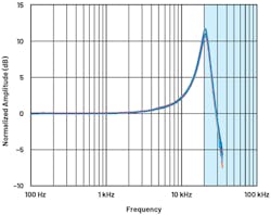
The frequency response plot for the ADXL1002 MEMS accelerometer is shown in Figure 1. The ADXL1002 3-dB bandwidth is 11 kHz, and it has a 21-kHz resonant frequency. A protective enclosure used to house the ADXL1002 needs to have a first natural frequency of 21 kHz or greater.

1. The ADXL1002 MEMS accelerometer frequency response.

Vibration Sensor Enclosure Model

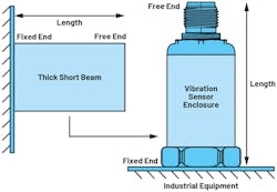
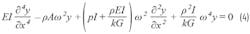
For modal analysis and design, a vibration sensor can be seen as a thick, short, cantilevered beam cylinder. In addition, the Timoshenko equation of vibration will be used for the simulation. This is covered in more detail later in the article.

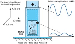
A thick, short, cantilevered cylinder is similar to a vibration sensor mounted on industrial equipment (Fig. 2). The vibration sensor is fixed to industrial equipment using a stud mount. Both stud mounting and enclosure design require careful characterization so that mechanical resonances don’t affect the MEMS vibration frequencies of interest. Finite element methods (FEMs) using Ansys or similar programs can be used as an efficient solver for the equation of vibration of a short, thick cylinder.

2. Modeling for a vibration sensor enclosure.

For modal analysis, Ansys and other simulation tools assume harmonic motion for every point in the design. The displacement and acceleration of all points in a design are solved as eigenvalues and eigenvectors—in this case, natural frequencies and mode shapes.

Natural Frequency and Mode Shape

The mass matrix M, stiffness matrix K, angular frequency ω_i, and mode shape {Φ_i} are related by Equation 1, which is used in FEM programs like Ansys.¹ The natural frequency f_i is calculated by dividing ω_i by 2π, and the mode shape {Φ_i} provides the relative deformation patterns of the material at specific natural frequencies:

For a single degree of freedom system, the frequency is simply expressed by:

Equation 2 provides a simple, intuitive way to evaluate a design. As you reduce the height of the sensor enclosure, the stiffness increases and the mass decreases—therefore, the natural frequency increases. Furthermore, as you raise the height of the enclosure, the stiffness reduces and the mass increases, resulting in a lower natural frequency.

Most designs have multiple degrees of freedom. Some designs have hundreds. Using the FEM provides quick calculations for Equation 1, which would be very time-consuming to do by hand.

Mode Participation Factor

The mode participation factor (MPF) is used to determine which modes and natural frequencies are the most important for your design. The mode shape {Φi}, mass matrix M, and excitation direction vector D are related by Equation 3¹ solving for MPF. The square of the participation factor is the effective mass:

The MPF and effective mass measure the amount of mass moving in each direction for each mode. A high value in a direction means the mode will be excited by forces, such as vibration, in that direction.

Using the MPF in conjunction with the natural frequency will enable the designer to identify potential design problems. For example, the lowest natural frequency produced by a modal analysis may not be the biggest design problem. That’s because it may not have as large a participation factor in your direction of interest (x-, y-, or z-axis plane) relative to all other modes.

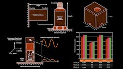
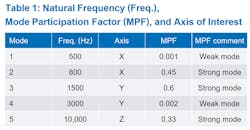
The examples shown in Table 1 illustrate that while a 500-Hz natural frequency is predicted in simulation for the x-axis, the mode is weakly excited and unlikely to be a problem. An 800-Hz strong mode is excited in the enclosure x-axis and will be a problem if the MEMS sensitive axis is oriented in the enclosure x-axis. However, this x-axis strong mode at 800 Hz isn’t of interest if designers have their MEMS sensor PCB oriented to measure in the enclosure z-axis.

Interpreting the Modal-Analysis Results

From the previous section, we know that modal analysis will indicate the natural frequencies in your axis of interest. In addition, the MPF will enable the designer to decide if a frequency can be ignored in a design. To complete the interpretation of modal analysis, it’s important to understand that all points on a structure vibrate at the same frequency (global variable), but the amplitude of vibration (or mode shape) at each point is different.

For example, an 18-kHz frequency can affect the top of the mechanical enclosure more than the bottom. The mode shape (local variable) has a stronger amplitude at the top of the enclosure compared to the bottom (Fig. 3). This means that while the enclosure structure’s top part is strongly excited by an 18-kHz frequency, the MEMS sensor at the enclosure bottom also will be affected by this frequency, though to a lesser degree.

3. A vibration sensor enclosure’s natural frequency, mode shape in axis of interest, and relative amplitude at the top and bottom of the enclosure.

Timoshenko Differential Equation of Vibration

The Timoshenko equation is suitable for modeling thick, short beams or beams subject to multi-kilohertz vibration. A vibration sensor (Fig. 2, again) is analogous to a thick, short cylindrical cross section, which can be modeled using the Timoshenko equation. The equation is a fourth-order differential equation with analytical solutions for restricted cases.

The FEM, as presented in Equation 1 to Equation 3, provides the most convenient method of solving the Timoshenko equation using multidimensional matrices. These scale with the number of degrees of freedom of the design.

Governing Equation

While FEM provides significant benefits in solving the Timoshenko equation of vibration in an efficient manner, an understanding of the tradeoffs in designing a vibration sensor enclosure requires closer examination of the Equation 4² parameters:

Using different materials or geometries will affect the natural frequency (ω) of the designed structure.

Material and Geometry Dependencies

The Timoshenko equation parameters can be grouped as either geometry dependent or material dependent.

Material dependencies are:

Young’s modulus (E): This is a measure of the elasticity of a material—how much tensile force is required to deform it. A tensile deforming force occurs at right angles to a surface.
Shear modulus (G): This is a measure of the shear stiffness of a material—the ability of an object to withstand a shear stress deforming force when applied parallel to a surface.
Material density (ρ): Mass per unit volume.

Geometry dependencies are:

Shear coefficient (k): While shear is a material property, the shear coefficient accounts for the variation of shear stress across a cross section. This is typically equal to 5/6 for a rectangular and 9/10 for a circular cross section.
Area moment of inertia (I): A geometrical property of an area that reflects how the geometry is distributed around an axis. This property provides insight into a structure’s resistance to bending due to an applied moment. In modal analysis, this could be considered as resistance to deformation.
Cross-sectional area (A): The cross-sectional area of a defined shape, such as a cylinder.

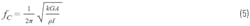
The Timoshenko equation predicts a critical frequency (f_C) given by Equation 5.³ As Equation 4 is fourth order, there are four independent solutions below f_C. For analytical purposes, the Equation 5 f_C is useful for comparing different enclosure geometries and materials.

A variety of approaches and solutions are available to determine all frequencies below f_C. Some approaches are noted in “Free and Forced Vibrations of Timoshenko Beams Described by Single Difference Equation”³ and “Flexural Vibration of Propeller Shafts Using Distributed Lumped Modeling Technique.”⁴ These approaches involve multidimensional matrices, like the FEM.

What Material Should I Use for My Design?

Table 2 details some common industrial metallic materials such as stainless steel and aluminum. Copper is the heaviest material of all four listed, and it doesn’t provide any advantage over stainless steel, which is lighter, stronger, and less expensive.

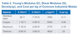
Aluminum is a good choice for weight-sensitive applications. Its density is 66% less than steel. The downside is that aluminum costs 20X more than steel per kilogram. Steel is the clear choice for cost-sensitive applications.

Although titanium is about two-thirds heavier than aluminum, its inherent strength means that you need less of it. However, using titanium is cost prohibitive for all but the most specialized weight-saving applications.

Simulation Example

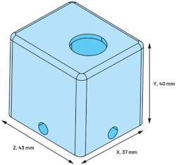
Figure 4 shows a 40- (H) × 43- × (L) 37-mm (W) rectangular metallic vibration sensor enclosure design. For modal analysis, the bottom surface (z, x) is a fixed constraint.

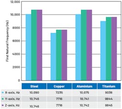
4. Rectangular enclosure with material type changed for simulation study.

Modal FEM analysis results for various enclosure materials are shown in Figure 5. The first natural frequency with significant MPF (greater than 0.1 for the ratio of effective mass to total mass of the system) is plotted vs. material type. It’s clear that aluminum and stainless steel have the highest first significant natural frequency. They’re also good material choices for low-cost or low-weight applications.

5. Rectangular enclosure with material type and first significant natural frequency (Hz).

Part 2 of the series covers whether to use a rectangular or cylindrical enclosure, maximum recommended height, the effect of wall thickness, and the impact of orientation on performance.

Read more articles in the Analog series: How to Design a Good Vibration Sensor Enclosure

References

1. ANSYS Innovation Courses: Modal Analysis. ANSYS, 2021.

2. Stephen Timoshenko. Vibration Problems in Engineering, 4^thedition. John Wiley and Sons Inc., New York, 1974.

3. Leszek Majkut. “Free and Forced Vibrations of Timoshenko Beams Described by Single Difference Equation.” Journal of Theoretical and Applied Mechanics, Vol. 47, No. 1, January 2009.

4. Mohammad Hossein Abolbashari, Somayeh Soheili, and Anoshirvan Farshidianfar. “Flexural Vibration of Propeller Shafts Using Distributed Lumped Modeling Technique.” The 16^thInternational Congress on Sound and Vibration, Krakow, 2009.

5. Saida Hamioud and Salah Khalfallah. “Spectral Element Analysis of Free - Vibration of Timoshenko Beam.” International Journal of Engineering, 2018.