How to Build Wide-Dynamic-Range Systems (Part 1)
Members can download this article in PDF format.
What you'll learn:
- Essentials for constructing a wide-dynamic-range system, including the application of switching or adaptive systems.
- Comparing multichannel vs. linear receivers.
- Analysis of how models react with different signal types.
For Part 2, click here.
The dynamic range of receiver devices is an important parameter that determines their ability to receive and process signals of varying power levels. Wide dynamic range is crucial in many fields, such as wireless communication systems, medical imaging devices, radar systems, and various probing systems. In practice, detecting weak signals amidst strong interference or noise is often necessary, and that requires a wide dynamic range.
In Part 1, we’ll explore methods for building systems with a large dynamic range and perform a comparative analysis of linear and multichannel receivers.
Constructing Wide-Dynamic-Range Systems
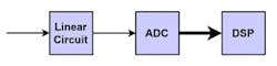
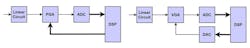
The dynamic range of modern radar, optoelectronic, and measurement systems spans from 80 to 160 dB. Various circuit solutions are employed to achieve such a wide dynamic range for amplification and measurement devices. Examples of these solutions include linear and superlinear systems and devices (Fig. 1). Being relatively simple to implement, they can give up to 100 dB of dynamic range.
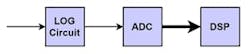
Devices with functional amplitude characteristics (Fig. 2) use the functional dependency between the input and output signals. Among devices with functional amplitude characteristics, those with logarithmic amplitude characteristics are the most common and can effectively compress the dynamic range. Fairly accurate logarithmic amplitude characteristics are achieved by implementing semiconductor diodes and transistors into the load or feedback circuits. These devices efficiently achieve a dynamic range of order of 106 to 1012.
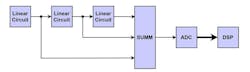
Devices with polygonal amplitude characteristics (Fig. 3) provide a good approximation to required functional dependencies, particularly those that are logarithmic. Such amplitude characteristics are typically achieved by summing the output signals from intermediate amplifier stages.
The most important and widely used method for expanding the dynamic range is the application of switching or adaptive systems (Fig. 4). With each switch, the gain coefficient of the system is adjusted so that the output signal always remains within the linear operating range of the analog-digital converter (ADC). The dynamic range expansion is achieved by increasing the number of switches. This method is widely used in measurement equipment for manual range switching of measurement conversion and in adaptive systems with automatic sub-range selection or adjustment of the transmission coefficient of the system.
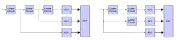
Multichannel systems, including systems with multichannel ADCs (Fig. 5), allow for expanding the dynamic range (similar to switching systems) and avoiding information loss, additional noise, and distortions caused by switching. By utilizing multiple channels simultaneously, these systems can handle a wider range of signal amplitudes without the need for switching, ensuring accurate and reliable signal acquisition.
Devices with logarithmic amplitude characteristics are considered the most optimal as they provide a large dynamic range and the lowest relative error within that range. Alongside devices with dynamic range switching or adaptive tuning, similar results are achieved by less widely adopted systems with multichannel ADCs. However, these systems have significant advantages that we’ll highlight in this article. The methods of expanding the dynamic range of receivers have been well explored by Iliin G.E. (1989).1
Simulating Receiver Devices with a Wide Dynamic Range
To compare receiver device characteristics, we created two models: a classical linear receiver and a multichannel ADC-based receiver. Figure 6 shows the structural diagrams for both. We assumed a dynamic range of 96 dB, which corresponds to a 16-bit ADC, for both models to make them easier to understand and implement.
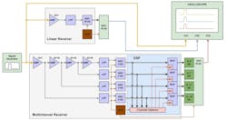
The models operate in the following way: The generator produces signals of various shapes, frequencies, and amplitudes, which are simultaneously fed to linear and multichannel receivers.
The linear receiver operates according to the classical scheme and doesn’t require further explanation.
The multichannel receiver has a dynamic range divided into four subranges so that each subsequent ADC, starting from the ADC1, is more sensitive than the previous one. This is achieved through a multi-stage connection of amplifiers, where the output of each amplifier is fed to the corresponding ADC channel.
For this scheme, it’s crucial that the amplifiers have a small saturation region and exhibit characteristics similar to an ideal limiting amplifier. ADC1 processes the most powerful signals with voltages ranging from Umax to Umax/16, while the other ADCs are in an overflow state. If the signal is in the range from Umax/16 to Umax/256, ADC2 is active. If it falls within the range from Umax/256 to Umax/4096, ADC3 is active. Finally, if the signal falls within the range from Umax/4096 to Umax/65536, ADC4 becomes active.
Depending on the signal level, the channel selector chooses only one ADC and passes its data through the enabled buffer corresponding to its group of digital-to-analog converter (DAC) bits. At the same time, the remaining channel buffers are disabled.
Influence of Various Signals on the Receiver Model
Let’s compare the advantages and disadvantages of the multichannel versus linear receiver by testing them in different operating modes. To accomplish this, we analyze how models react to signals with different shapes and amplitudes.
Analyzing the influence of the ramp signal
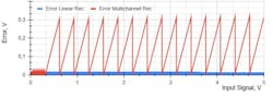
The primary purpose of this test is to evaluate the absolute measurement error of the receivers. To provide this test, we’ll generate a ramp signal (Fig. 7) and pass it through the models.
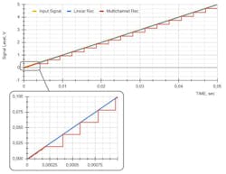
Since the multichannel receiver forms the resulting signal only from one ADC during each clock cycle, it’s evident that the measurement error should be higher. As depicted in Figure 7, the "step" size increases as the input signal rises.
Figure 8 illustrates the relationship between the absolute measurement error and the input signal level. As anticipated, the absolute measurement error remains constant throughout the dynamic range for the linear receiver, equaling half the value of the least significant bit of the ADC. However, the situation is quite different for the multichannel receiver, because the measurement error depends on the specific subrange in which the receiver is currently operating.
Analyzing the influence of the sinusoidal signal
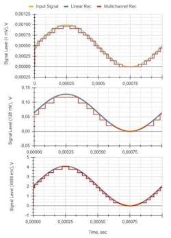
The primary purpose of this test is to evaluate the mean squared error (MSE) of the measurement when a sinusoidal signal propagates through the receiver model (Fig. 9).
To obtain an objective result, we generated sinusoidal signals of various amplitudes and calculated the MSE each time using the following formula:
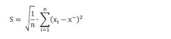
Similarly, regarding the case of a linearly changing signal, the "step" size depends on the amplitude. At low signal levels, the quantization step for both the linear receiver and the multichannel receiver is the same. This is reflected in the MSE dependency on the signal level shown in Figure 10, where the errors are almost equal.
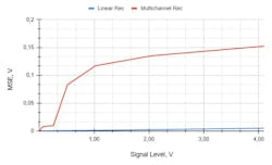
As the signal amplitude increases, the processing channels change in the multi-channel receiver, which affects the MSE and causes it to increase. In contrast, the MSE of the linear receiver is practically independent of the signal level and remains constant throughout the dynamic range. Thus, the measurement error of the multichannel receiver is higher compared to the linear receiver.
Analyzing the influence of the pulse signal
The multichannel receiver with a divided dynamic range has advantages compared to the linear receiver. Let’s examine the behavior of the models under the influence of pulse signals.
As is known, signals undergo linear distortions when passing through filtering circuits. These distortions can be observed as rounded edges when the bandwidth is limited from above and as a droop in the flat part of the pulse when the bandwidth is limited from below.
In the models, the anti-aliasing filter serves as the filtering element to improve signal digitization quality and eliminate the effect of spectrum overlap. In our model, the anti-aliasing filter is implemented in such a way as to provide a 20-dB attenuation at a frequency of 0.6 × Fsample, and a 30-dB attenuation at the sampling frequency Fsample.
After passing the pulse signal through the receiver model, we can see the following pattern (Fig. 11). The input signal to the receivers is highlighted in yellow, the output signal of the linear receiver is shown in blue, and the output signal of the multichannel receiver is shown in red. The output pulse signals are almost similar and have rounded edges, which is consistent with the theory of electrical circuits. Visually, the only difference is that the output signal of the multichannel receiver has an error in measuring the flat portion of the pulse peak. The cause of this error was described earlier.
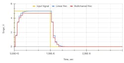
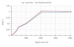
Figure 12 shows the dependency of the MSE on the level of the pulse signal applied to the input of the receiver model. The MSE in this case is nearly identical. Undoubtedly, if the bandwidth, pulse duration, or sampling frequency is changed, the integral error will also change, but the situation fundamentally remains the same.
Building and Analyzing Wide-Dynamic-Range Systems
This article explored several approaches for constructing high-dynamic-range systems. Dynamic-range values were provided for each of these approaches. Based on the review, two options were chosen for modeling and conducting a comparative analysis: a linear system and a multichannel system with dynamic range partitioning. The primary evaluation criterion was MSE while passing through receiver models using different signals.
When passing a ramp signal, it was determined that the MSE of the linear receiver remained constant, whereas in the multichannel receiver, it increased as the signal level grew. A similar trend was observed when passing sinusoidal signals through receiver models of varying levels. However, when testing with impulse signals, the error was nearly consistent across the entire amplitude range.
Thus, the multichannel receiver demonstrated higher MSE values for ramp and sinusoidal signals, and nearly identical values for impulse signals when compared to the linear receiver. However, by utilizing a multichannel receiver, a significant extension of the dynamic range can be achieved compared to the linear counterpart.
The multichannel receiver finds its application in systems where impulse signals prevail, such as radar systems in various fields.
Reference
1. Iliin, G.E., Polskij, J.E. (1989) “Dynamic range and accuracy of radio electronic and optoelectronic measuring system. Results of science and technology,” Radiotehnika series, 39, 67-114.
About the Author
Petr Liutuk
Petr Liutik has over a decade of experience developing software for various embedded systems. He started his career by working on wireless fire alarm systems and intelligent home systems based on 802.15.4 and Zigbee technologies. Later, he engaged in software development for a programmable logic controller running on the QNX operating system and implemented CODESYS support. Petr also participated in porting and developing the Linux-based mobile operating system Aurora/Sailfish.
Konstantin Liutuk
Konstantin Liutik is an experienced engineer with a strong background in analog and digital electronics, circuits, and PCB design. He has expertise in developing low-power microwave transmitters, receivers, and antenna switches. In addition, he has experience designing high-speed multilayer PCB topologies using Mentor Graphics CAD and signal-integrity analysis tools such as HyperLynx.
Comment About the Article
To join the conversation, and become an exclusive member of Electronic Design, create an account today!

Leaders relevant to this article: