Eigenvalues Provide Insight into Power-Supply Filter Performance
This file type includes high resolution graphics and schematics when applicable.
Switch-mode power supplies based on pulse-width modulation (PWM) have been in use since the early 1970s. One of their key circuit blocks has received relatively less attention, though: the second-order LC filter fed by the PWM wave. The role of this block is to extract the dc power embedded in the pulse train, and to suppress the undesirable harmonics to the extent possible. For the latter function, which is seen as a complex periodic ripple, it’s desirable to have a speedy approach capable of zeroing in on the steady-state ripple.
One way to do that is by using eigenvalues, which sounds esoteric but are quite useful. Eigenvalues (from the German meaning "their own values") are a special set of scalars associated with a linear system of equations such as matrix equations. They’re also called characteristic roots or characteristic values.
An LC Filter with PWM Drive
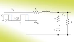
A loaded LC filter driven by a PWM pulse train contains numerous parasitic elements (Fig. 1).
There are two state variables—inductor current i and capacitor voltage v. The state equation that represents the operation of the filter driven by a PWM voltage source, Eg, is:
where Rp represents rc and R in parallel, and kR = R/(rc+R). The solution to this state equation is:
The second form is applicable for a constant driving source, which is generally the case for switch-mode dc-dc converters. Furthermore, during the active on-time, nTs < t < (n+D)Ts, so
and during the off-time, (n+D)Ts< t < (n+1)Ts, with
Given two as-yet unknown starting states X1 and X2 at t = nTs and t = (n+D)Ts, the continuity of states requires that, at t = (n+D)Ts and t = (n+1)Ts:
Combining Equations 5 and 6 yields:
The Role of Eigenvalue
The key to resolving the above equation is the computation of matrix exponentials, such as eA1 and eA2. From basic linear algebra, a 2 × 2 matrix A1 (or A2) has characteristic equations:
|A1-λ1I|=0 or |A2-λ2I|=0]
with two eigenvalues, λ11 and λ12 (or λ21 and λ22).The Cayley-Hamilton Theorem states that:
Therefore:
and so the cyclic starting states X1 and X2 are no longer unknown.
The computation for eAt is slightly more demanding. In this case, eAt = β0(t)+ β1(t)A with two new eigenvalues, again represented by λ1 and λ2 , for matrix A of Equation 1. Therefore:
which concludes the computation of the two alternating solutions, Equations 3 and 4, in steady state for the filter driven by a periodic PWM pulse train.
An example illuminates the analysis. If L = 102 μH, rL = 0.005, C = 100 μF, rC = 0.01, R = 2.12, Ts = 8 μs, D = 0.329, Vs = 17.184, and VD = 0.5, then system transition matrix:
and auxiliary matrix A1=ADTs, A2=A(1-D)Ts:
define the two eigenvalues for each matrix A1 and A2:
Using Equation 9 yields:
and Equation 8 gives eA1 and eA2. Then Equations 7 and 5 give the cyclic starting states as:
For the two eigenvalues of A (λ1 and λ2):
Equation 10 and eAt = β0(t) + β1(t)A follow, leading to steady-state solutions for DTs and (1-D)Ts time segments in one cycle:
Graphical plots of the inductor current and the output voltage over five cycles make the results of the equations clear (Fig. 2). Figure 3 gives an actual measurement that matches well with the Figure 2 computation.
Keng C. Wu, Switching Power Inc., holds a BS from Chiaotung University, Taiwan, and an MS from Northwestern University, Evanston, Ill. He has published four books and holds 12 U.S. patents.
About the Author
Voice Your Opinion!
To join the conversation, and become an exclusive member of Electronic Design, create an account today!

Leaders relevant to this article:


