Stability Criteria Of A Control System

In the electronic field, an oscillator is a circuit capable of producing a self-sustained sinusoidal signal. In a lot of configurations, cranking up the oscillator involves the noise level inherent to the adopted electronic circuit. As the noise level grows at power-up, oscillations are started and self-sustained. This kind of circuit can be formed by assembling blocks such as those appearing in Fig. 1. As you can see, the configuration looks very similar to that of our control system arrangement.
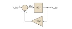
In our example, the excitation input is not the noise but a voltage level, Vin, injected as the input variable to crank the oscillator. The direct path is made of the transfer function H(s), while the return path consists of the block G(s). To analyze the system, let us write its transfer function by expressing the output voltage versus the input variable:

If we expand this formula and factor Vout(s), we have

The transfer function of such a system is therefore

In this expression, the product G(s)H(s) is called the loop gain, also noted T(s).To transform our system into a self-sustained oscillator, an output signal must exist even if the input signal has disappeared. To satisfy such a goal, the following condition must be met:

To verify this equation in which Vin disappears, the quotient must go to infinity. The condition of the quotient to go to infinity is that its characteristic equation, D(s), equals zero:
1+ G(s)H(s) = 0 (5)
To meet this condition, the term G(s)H(s) must equal -1. Otherwise stated, the magnitude of the loop gain must be 1 and it sign should change to minus. A sign change with a sinusoidal signal is simply a 180° phase reversal. These two conditions can be mathematically noted as follows:
|G(s)H(s)| = 1 (6)
ArgG(s)H(s) = –180o (7)
3.2 Stability Criteria
You understand that our goal with a control system is not to build an oscillator. We want a control system featuring speed, precision, and an oscillation-free response. We must therefore keep away from a configuration where conditions for oscillation or divergence are met. One way is to limit the frequency range within which our system will react. By definition, the frequency range, or the bandwidth, corresponds to a frequency where the closed-loop transmission path from the input to the output drops by 3 dB. The bandwidth of a closed-loop system can be seen as a frequency range where the system is said to satisfactorily respond to its input (i.e., follows the setpoint or efficiently rejects the perturbations). As we will later see, during the design stage, We do not directly control the closed-loop bandwidth but the crossover frequency fc, a parameter pertinent to an open-loop analysis. Both variables are often approximated as equal, and we will see that it is true in one condition only. However, they are not far away from each other, and both terms can be interchanged in the discussion.
Related Articles
- Understanding the Right-Half-Plane Zero Part 1
- Understanding the Right-Half-Plane Zero
- Eliminate the Guesswork in Selecting Crossover Frequency
- New Technique for Non-Invasive Testing of Regulator Stability
We have seen that the open-loop gain represents an important parameter for our control system. When gain exists (i.e. |T(s)|>1), the system works in dynamic closed-loop conditions and can compensate for incoming perturbations or react to setpoint changes. However, there is a limit to the system reaction: the system must offer gain at the frequencies involved in the perturbing signal. If the perturbations of the setpoint changes are too fast, the frequency content of the excitation signal is beyond the bandwidth of the system, implying the absence of gain at these frequencies: the system becomes slow and cannot react, operating as if the loop were unresponsive to varying waveforms. Is an infinite bandwidth system desirable then? No, because increasing the bandwidth is like widening the diameter of a funnel: you are certainly going to collect more information and react faster to incoming perturbations, but the system will also accept spurious signals such as noise and parasitic data, self-produced by the converter in some cases (the output ripple in switching power supplies, for instance). For this reason, it is mandatory to limit the bandwidth to what your application really requires. Adopting too wide a bandwidth would be detrimental to the noise immunity of the system (e.g. its robustness to external parasitic signals).
LIMITING BANDWIDTH
How do we limit the bandwidth of a control system? By shaping the loop gain curve through the compen or block, G. This block will make sure that after a certain frequency fc, the loop gain magnitude |T(fc)| drops and passes below 1 or 0 dB. As we explained, it is roughly the bandwidth of your control system once the loop is closed. The frequency at which this phenomenon occurs is called the crossover frequency noted fc. Is this enough to obtain a robust system? No, we need to ensure another important parameter: The phase of T(s) at the point where its magnitude is 1 must be less than -180°. From our experiments, we have seen that when the loop phase is less than -180° at the crossover frequency, we obtain a response converging toward a stable state. This is obviously a highly desirable characteristics of our control system. To make sure we stay away from the -180° at crossover, the compensator G(s) must tailor the loop argument at the selected crossover frequency to build phase margin, PM or φm. The phase margin can be considered a design or a safety limit ensuring that despite external perturbations or unavoidable production spreads, changes in the loop gain will not put the stability in jeopardy. As we will later see, the phase margin also impacts the transient response of the system. Therefore, its choice does not exclusively depend on stability considerations but also the type of transient response you want. Mathematically, the phase margin is defined as follows:
φm= 180 + ∠T(fc) in degrees (8)
where T represents the open-loop gain made of the cascaded plant H and compensator G gains.
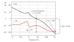
A typical compensated loop gain curve appears in Fig. 3 and shows a crossover frequency of 6.5 kHz. At this point, the phase of T(s) is -90°. If you start from the -180° at a 6.5-kHz frequency and positively count the degrees until you cross the argument wave form, you have the phase margin: 90° in this example. This is an extremely robust system that is told to be unconditionally stable : despite moderate loop gain variations around the crossover point, there are no possibilities to cross over at a frequency where the phase margin is too small. By too small, we mean a phase margin approaching 30°, a limit below which the system gives an unacceptable ringing response. This is the reason why you learned at school that 45° was the limit, giving an extra margin compared to 30°. We will later see that there is an analytical origin for these numbers.
Gain Margin and Conditional Stability
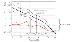
Fig. 4 shows another typical frequency response of a compensated converter, highlighting the 0-dB crossover point as well as the phase margin. We know by experience that the elements constitutive of the converter will exhibit variations along the product life cycle. These variations can be linked to natural production spreads (for instance, resistors or capacitors affected by lot-to-lot tolerance). The converter environmental operating conditions also have an impact on components. Among these variables, temperature plays an important role and affects passive or active component parameters. It can be capacitors or inductors equivalent series resistors (ESR), the optocoupler current transfer ratio (CTR), or the beta of bipolar transistors for instance. These variations impact the loop gain by shifting it up or down depending on the affected parameters.
If the gain curve undergoes a shift, the 0-dB crossover frequency will transition to a new value imposing a different bandwidth to the converter. How can the converter stability be affected under these changes? Well, if the new crossover tales place at a point where the phase margin is weak, you may degrade the transient response so that the overshoot is no longer acceptable. It is thus your responsibility, as a designer, to ensure that these dispersions do not suddenly increase the gain at a frequency where you approach the -180° limit. You need sufficient gain margin as defined by

Where ƒncorresponds to the frequency point where is exactly -180° or radians (1 MHz in Fig. 3).
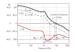
Fig. 4 portrays typical gain variations of ±10 dB due to production spreads in the selected components. It brings the crossover frequency from 1.5 kHz to 30 kHz. In this area, the phase margin changes from 70° to 45°, safe numbers according to theory. What is the worst case? It is when the new crossover frequency occurs where the total phase lag is 180°, matching the conditions for oscillations. This condition occurs at 1 MHz, implying a positive gain change of 35 dB.
LARGE GAINS UNLIKELY
Fortunately, deviations of 35 dB are unlikely to happen in modern electronics circuits. Time ago, when amplifiers or servomechanisms were driven by vacuum tubes-based circuits, warm-up times during the power-on sequence could induce large loop gain variations. Gain provisions were thus necessary to reject a second point where the stability could be in danger. This gain margin, identified on the loop gain curve at the frequency where the total phase lag reaches -180°, is noted GM in Fig. 3. In modern electronic circuits, gain margins beyond 10 dB are usually enough, unless your loop gain exhibits extreme sensitivity to an external parameter.
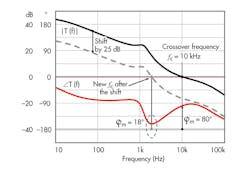
Another example of gain shift appears in Fig. 5. It shows another compensated converter exhibiting a phase margin of 80° at 10 kHz. Based on what we discussed, we know that gain changes can occur, inducing ups or downs on the gain curve. In our example, we can identify an area around 2 kHz where the phase margin is as small as 18°. If a gain decrease of 20-25 dB occurs, you can end up with a control system showing a dangerously low phase margin around 2 kHz. It would lead to an oscillatory response, perhaps exceeding the overshoot specifications. This kind of system is told to be conditionally stable. Fortunately, as already said, a 25-dB variation of gain is unusual and such a system can be considered robust with this gain margin. However, I have seen design cases where the end user (your customer) clearly stated in the specifications that conditional designs were not acceptable, asking for a phase margin greater than 60° at all points below the crossover frequency. In this case, it becomes mandatory to compensate the converter so that no region of reduced phase margins below crossover ever exist whatever the operating conditions are.
Stable or Unstable?
It is often believed that a system where the phase dips below -180° before crossover is an unstable system. Such a response appears in Fig. 6. The phase curve quickly drops after 1 kHz and passes the -180° limit at 1.5 kHz for a few kilohertz.
It then goes up again to offer a phase margin of 50° at 10 kHz. Yes, this system is stable simply because we do not satisfy (3.7) at 0 dB. Remember, to cancel the denominator of (3.3), you must have the gain magnitude exactly equal to 1 and a phase lag of 180° or beyond. In the graph, we can see that this condition is not satisfied at any point in the picture. However, it is worth noting that the loop is highly conditional. Should the gain reduce by a few decibels and your phase margin becomes less than 45°. Another 10-dB decrease and you enter a dangerous area of zero phase margin where, this time, the oscillation criteria would be met.
Note: This article is reprinted from the book “Designing Control Loops for Linear and Switching Power Supplies: A Tutorial Guide,” (c) 2012, with permission of the publisher, Artech House, Inc., Boston. The subjects in the book include: Basics of Loop Control, Transfer Functions, Stability Criteria of a Control System, Compensation, Operational Amplifier-Based Compensation, Operational Transconductance Amplifier-Based Compensation, TL-431-Based Compensation, Shunt Regulator-Based Compensation, Measurements and Design Examples. The book can be purchased at ArtechHouse.com, Amazon.com, or BN.com
About the Author
Christophe Basso
Christophe Basso is a Technical Fellow at ON Semiconductor in Toulouse, France, where he leads an application team dedicated to developing new offline PWM controller specifications. He has originated numerous integrated circuits among which the NCP120X series has set new standards for low standby power converters.
Further to his 2008 book “Switch-Mode Power Supplies: SPICE Simulations and Practical Designs”, published by McGraw-Hill, he released in 2012 a new title with Artech House, “Designing Control Loops for Linear and Switching Power Supplies: a Tutorial Guide”. His new book is dedicated to Fast Analytical Techniques and was recently published by Wiley in the IEEE-press imprint under the title “Linear Circuit Transfer Function: An Introduction to Fast Analytical Techniques”.Christophe has over 20 years of power supply industry experience. He holds 17 patents on power conversion and often publishes papers in conferences and trade magazines including How2Power and PET. Prior to joining ON Semiconductor in 1999, Christophe was an application engineer at Motorola Semiconductor in Toulouse. Before 1997, he worked as a power supply designer at the European Synchrotron Radiation Facility in Grenoble, France, for 10 years. He holds a BSEE equivalent from the Montpellier University (France) and a MSEE from the Institut National Polytechnique of Toulouse (France). He is an IEEE Senior Member.
Comment About the Article
To join the conversation, and become an exclusive member of Electronic Design, create an account today!

Leaders relevant to this article: