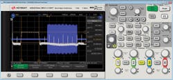
Scope FFT and waveform math functions take on RF measurements
In the process of debugging and validating both digital and RF designs, the oscilloscope Fast Fourier Transform (FFT) function and a variety of other math functions can prove valuable to designers moving beyond the prototype stage and into production. For example, with digital designs, the FFT function in an oscilloscope can quickly highlight the frequency content of signals that are making their way onto power supply rails and further pinpoint the source of such noise signals with that knowledge. That’s important because such signals can translate into noise in other parts of the design, cutting signal margins and potentially preventing the design from moving beyond the prototype stage until the problem is fixed.
An FFT spectral view also is helpful when looking at more complex, wide spectral signals to verify if the proper modulation is happening. Time-gated FFTs further evaluate spectral components of a signal. Math functions such as a frequency trend can quickly verify whether a classic modulation scheme is happening properly, like a linear frequency modulation across pulses in a stream. This article will explore a number of these examples and look at practical considerations for the measurements.
FFT measurement with an input sine wave
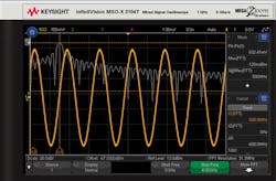
An oscilloscope that has a 1-GHz analog bandwidth and up to a 5-GS/s sample rate will be used for measurements. These are both important specifications that will tie into what kinds of measurement applications are possible. The first example measurement is the capture of a 600-MHz, 632-mV (p-p), 0-dBm, 1-mW sine-wave signal into 50 Ω (orange) and resultant FFT (white) as shown in Figure 1.
It’s important to understand how the oscilloscope sampling characteristics play into the quality of this FFT measurement. The oscilloscope analog bandwidth, sample rate, memory depth, and related time capture period all can have a profound effect on the measurement result. This effect is heavily influenced by the characteristics of the signal under test and how those signal characteristics are related to the oscilloscope capture performance.
For example, in this simple illustration of measuring a single-tone 600-MHz sine-wave signal and wanting to see the basic spectral characteristics of that signal, the oscilloscope has to have enough analog bandwidth to minimally attenuate the amplitude of the signal. Since this oscilloscope has a maximum 1-GHz analog bandwidth, there is plenty of oscilloscope bandwidth to measure the 600-MHz tone.
To avoid aliasing in the digitizing process, sampling must occur at a rate at least twice the frequency of any appreciable frequencies present in the signal under test. In this example, a 1.2-GHz sampling rate would be required. Clearly, if the scope is sampling at its maximum 5-GS/s rate, that is more than sufficient. However, it will be shown later that for certain scope time-base settings the sample rate (and bandwidth) will decrease.
So what kind of quality is there in the FFT measurement made on the 600-MHz sine wave? Referring back to the oscilloscope FFT measurement in Figure 1, notice the main single frequency spike with a related measurement marker showing around a 600-MHz frequency and 0-dBm power. That matches expectations, but the FFT response looks very wide for a single frequency input signal.
The spacing between frequency spectrum lines in the FFT, or the width of frequency buckets that signal energy is apportioned to, is called the frequency resolution. It is based strictly on the time length of the acquired data and a factor for the FFT windowing type selected. A rectangular window is used here with a factor of 1, so the frequency resolution is simply the inverse of the record time. In this example:
Frequency Resolution = 1/(1 ns/div x 10 div) = 100 MHz
So this FFT could distinguish frequency components in the signal spectrum as close as 100 MHz, but any components closer than 100 MHz apart would merge together and be indistinguishable. That’s actually a really coarse measurement.
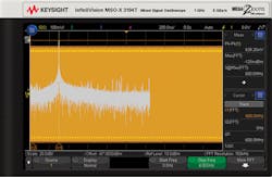
How an increased time on screen enhances the FFT response
To demonstrate the importance of the record time upon FFT results, if the time/division is panned to 200 ns/div, with a new record time of 2 μs across the screen, the frequency resolution changes drastically to:
Frequency Resolution = 1/(200 ns/div x 10 div) = 500 kHz
The significant change in the FFT result can be seen in Figure 2 with a much finer display of the 600-MHz frequency-domain spike. A trade-off is happening here. More time samples are being processed, the calculated FFT has more spectral lines, and better frequency resolution results. But the measurement runs slower than before to process more data—10,000 samples instead of the original 50.
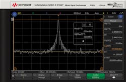
Start-frequency, stop-frequency, center-frequency, and span controls
An important capability in the FFT calculation and resultant view is to be able to zoom into an area of interest for analysis. The first example had a wide span from 0 Hz to 2.5 GHz, so it was difficult to see any detail around the 600-MHz carrier. Suppose there was suspected noise around the 600-MHz carrier frequency and a desire to inspect that. The FFT controls can set a center frequency at 600 MHz and a desired span, such as 100 MHz, around the 600-MHz carrier. A start frequency of 550 MHz and stop frequency of 650 MHz also could have been selected with the same result. An FFT measurement with these parameters can be seen in Figure 3.
Wideband FFT analysis
An increasing number of today’s signals have modulation present that can increase the spectral width to hundreds of megahertz or even multiple gigahertz. If spectral widths of signals are beyond around 500 MHz, then spectrum analyzers or vector signal analyzers available today do not have enough analysis bandwidth to make meaningful measurements. In such cases, an oscilloscope or digitizer is required that has enough analysis bandwidth for the application.
The carrier frequency of a signal of interest also is important. The carrier frequency of the signal under test plus half the spectral width of that signal must be less than or equal to the oscilloscope bandwidth for the oscilloscope to be used on its own for the measurement. A wideband signal frequency domain measurement will now be considered.
The signal under test is a 600-MHz RF pulse train, with 4-μs-wide RF pulses repeating every 20 μs. There is a linear frequency modulation of the signal that chirps the carrier frequency from 300 MHz at the start of the RF pulse envelope to 900 MHz at the end of the pulse envelope.
To make a basic FFT measurement of the RF pulse, the first step is to get a clean time-domain capture of a pulse from the signal on screen. The scope is reset to a known condition by pressing Default Setup. Then Auto Scale is pressed, and the time/division setting is adjusted to bring one main RF pulse on screen. The basic default rising-edge trigger is further qualified with trigger holdoff. This ensures that a trigger doesn’t happen mid-pulse since that would create instability in the captured trace. The trigger holdoff is set to something slightly longer than the width of the RF pulse. The RF pulse is 4 μs wide so a trigger holdoff of 5 μs works well.
Next the FFT button is pressed to calculate a spectral view of the RF pulse train from the time-domain digitized signal on screen. There are FFT controls for start and stop frequency or center frequency and span. A wide span is first chosen with a start frequency of 0 Hz and a stop frequency of 2.5 GHz. Since this is a pulse signal, and an entire pulse can be placed on screen with only noise on the left and right side of the scope screen, a rectangular window is chosen for the FFT calculation. FFT averaging with a count of eight also helps optimize the measurement result. The FFT response that results is shown in Figure 4.
Markers are placed on the FFT response, and it can be seen that this RF pulse does have a wide spectral width, from 300 MHz to 900 MHz, or 600 MHz wide. What’s not yet proven is that the frequency of the carrier shifts from 300 MHz to 900 MHz, linearly, from the left side of the pulse across to the right side of the pulse.
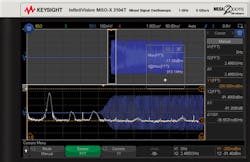
The gated FFT math function
One way to quickly see some carrier frequency values across the pulse is to use the gated FFT function. This is achieved by turning on the normal time-domain trace time gating function. This function generates a normal trace view at the top half of screen and a magnified view at the bottom of the screen. The time/division control expands and shrinks the time-gate window placed on the upper normal trace, and the time delay control moves the window along the trace. Whatever portion of the waveform is present in this window shows up in the lower trace, but magnified.
An interesting measurement results from creating a small time-width window at the very beginning of the pulse. The FFT is calculated from the data contained within the gated time window as shown in Figure 5.
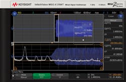
The FFT measurement of the peak value amplitude and frequency of the spike shows that the RF pulse begins with a carrier frequency around 300 MHz. If the time-gate window is moved to the center of the RF pulse, the frequency is seen to be around 600 MHz. And it is 900 MHz at the end of the RF pulse. This appears to be a linear frequency-modulated chirp as desired.
Frequency measurement and measurement trend math function
In some cases, a measurement trend math function can give a helpful view of the frequency chirp profile. The oscilloscope is able to display up to 1,000 measurements in a trend format. In a similar signal example, a 600-ns-wide pulse train, repeating every 20 μs, needs to be verified. The FFT function now is turned off, and purely time-domain measurements are made.
First, the acquisition mode of the oscilloscope is changed from Normal capture to High Resolution capture mode. Second, a frequency measurement is selected from the list of possible measurements, by pressing the Measure button. A middle threshold for carrier zero crossing detection is set to 30 mV given that the swing of the carrier signal is from around -316 mV to +316 mV (1-mW signal, 0 dBm into 50 Ω). Then the Math key is pressed, and a math function called measurement trend is chosen. Markers are assigned to have their source be the math function result. An interesting view of frequency measurements taken across the RF pulse can be seen in Figure 6.
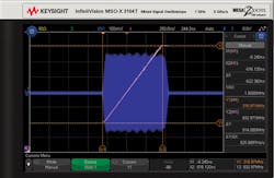
Clearly, the pulse carrier is shifting in a linear fashion across the pulse, from left to right, as designed. Notice that the linear ramp display is not going across the entire width of the RF pulse. This is because the 1,000 measurement limit in the trend calculation has been reached. It is important that a portion of the pulse FM function can be seen, and it is linear. For the frequency measurements across the pulse to have enough precision, it was imperative that the High Resolution acquisition mode was selected.
Summary
FFTs in oscilloscopes are a valuable tool to give a frequency-domain view of a signal. This can ultimately be done with very wide bandwidth, enabling measurements not possible with a narrower band vector signal analyzer. Example FFT measurements were able to verify that a linear FM chirp signal was shifting the carrier frequency as it should. There also was a place for other math functions, namely the measurement trend function. In this example, such a calculation allowed for a very simple verification of a linear FM chirp.
About the author
Brad Frieden is a product planner/product marketing engineer for the Oscilloscopes and Protocol Division of Keysight Technologies. He has been with HP/Agilent/Keysight for 30 years and involved in a variety of marketing roles in areas including fiber-optic test, pulse generators, oscilloscopes, and logic analyzers. Frieden received a B.S.E.E. from Texas Tech in 1981 and an M.S.E.E. from the University of Texas at Austin in 1991.
About the Author

Comment About the Article
To join the conversation, and become an exclusive member of Electronic Design, create an account today!

Leaders relevant to this article: