Current shunt power coefficient determination
Based on a Fluke Calibration paper1
Current often is derived from the voltage drop measured across a shunt of known value. However, as the paper states, “It is common practice for current shunts to be calibrated at a single current level and then used over a wide range of currents. The power coefficient (PC) of the shunt can contribute significant error to the measurement process. Often the power coefficient is ignored either through lack of awareness or because it is specified to be acceptably small. For many shunts, however, the power coefficient is far from insignificant and an accurate characterization can provide a set of power coefficient corrections that can significantly reduce measurement uncertainty.”
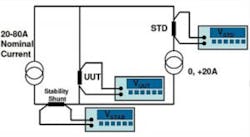
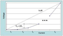
Given the obvious advantage provided by including the effect of a shunt’s PC, the problem then is to devise a means of measuring it. Several straightforward methods that require the use of a calibrated standard shunt are discussed in the paper. For example, connecting the unknown (UUT) and standard shunts in series, as shown in Figure 1, ensures that the same current passes through both. However, the currents I1 through I4, although small, are not zero. These bias currents must be low enough to have an insignificant effect on the measurement to the accuracy level required.

Direct comparison at different current levels is useful, but, as the paper’s authors noted, although the PCs of two shunts compared to within 2 or 3 µΩ/Ω between 10 A and 20 A, both shunts had about a 12-µΩ/Ω shift in value over that current range. Most likely, this was caused by the manganin alloy wire used in the shunt construction. Manganin exhibits a zero temperature coefficient (TC) at room temperature and a negative TC at both lower and higher temperatures.
New Approach
A new test setup devised both to provide accurate PC measurement as well as minimize the effects of reference shunt uncertainties is shown in Figure 2. Two current sources are used, one that changes its output in 20-A steps from 20 A to 80 A and the other switchable from zero to +20 A or -20 A. For each 20-A step in the first source, the other source is stepped through -20 A, zero, and +20 A, with voltage measurements across the UUT taken for each combination of currents. This method creates a series of readings taken “symmetrically in time about the UUT DMM readings.” The readings can be averaged to eliminate most of the effect of any drift in the values of the shunts.
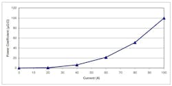
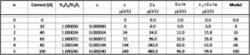
To demonstrate the procedure, the PC of a hypothetical 0.008-Ω 100-A UUT was evaluated. The STD shunt has a value of 0.01 Ω and the Stability shunt 0.001 W. It is assumed that the UUT PC is linear with power as shown in Table 1, with a value of 0.01 *I2 µΩ/Ω.
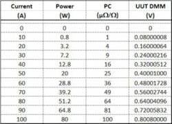
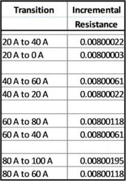
The entries in Table 2 were calculated using the nominal STAB and STD shunt values. Analysis of the data provides incremental values of UUT voltage vs. current. Dividing incremental voltage by incremental current gives the value of the incremental resistance, shown in Table 3. Figure 3 further defines the relationships among these quantities.


V1, V2 are incremental voltages caused by changes in current
I is the total current
e is the PC at the total current I: en is the PC at current In
R0 is the UUT shunt resistance value at low current; negligible PC

(Click image to enlarge)
(Click image to enlarge)

Working through the math using the R0 = V1/I1 approximation

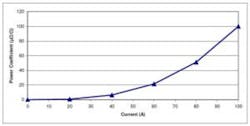
Table 4 demonstrates that the measurement method returned the expected PC values for the UUT in this experiment: it followed a current-squared curve as shown in Figure 4. Table 4 includes the post-analysis 4% correction—the 3.8 value for e1 is equal to 4% of 96—the total uncorrected power coefficient. Dividing the sum by 5 in the third column from the right hand end accounts for each Ij being only 1/5 of the total I.
(Click image to enlarge)
(Click image to enlarge)
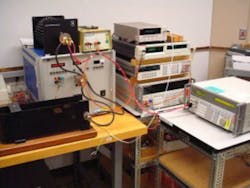
Figure 5 shows the actual test setup used to verify the square-law characteristic of the PC for a Fluke 100-A shunt.
Reference
- Deaver, D. and Faulkner, N., Characterization of the Power Coefficient of AC and DC Current Shunts, Fluke, 2010.
About the Author

Comment About the Article
To join the conversation, and become an exclusive member of Electronic Design, create an account today!

Leaders relevant to this article: