How to Model Statistical Tolerance Analysis for Complex Circuits Using LTspice
Members can download this article in PDF format.
What you'll learn:
- How to use statistical tools for component tolerance analysis.
- A look at methods such as Monte Carlo and Gaussian distribution.
- Simulating a dc-dc converter in LTspice to model closed-loop voltage feedback.
LTspice can be utilized to perform statistical tolerance analysis for complex circuits. To show the efficacy of the method, this article presents a voltage regulation example circuit modeled in LTspice, demonstrating Monte Carlo and Gaussian distribution techniques for the internal voltage reference and feedback resistors. The results of this simulation are compared to a worst-case analysis simulation.
Included are four appendices: Appendix A provides insights on the distribution of trimmed voltage references. Appendix B offers an analysis of the Gaussian distribution in LTspice. Appendix C provides a graphical view of the Monte Carlo distribution as defined by LTspice. Appendix D lays out instructions for editing LTspice schematics and extracting the simulated data.
This article is not a review of 6-sigma design principles, the central limit theorem, or Monte Carlo sampling.
Tolerance Analysis
In system design, parametric tolerance constraints must be considered to ensure a successful design. A common approach uses worst-case analysis (WCA) where all parameters are adjusted to their maximum tolerance limit. In a WCA, the performance of the system is analyzed to determine if the worst-case result lies within the system design specification. There are limitations to the efficacy of WCA, such as:
- WCA requires determining which parameters must be maximized or minimized for a true worst-case result.
- WCA results often violate design specification requirements, leading to expensive component selection to obtain acceptable results.
- WCA results statistically don’t represent commonly observed results; observing a system exhibiting WCA performance may require a very large number of assembled systems.
An alternate approach for system tolerance analysis is to use statistical tools for component tolerance analysis. The benefit of a statistical analysis is the resulting data has a distribution that reflects what should be commonly measured in physical systems. In this article, LTspice is used to simulate circuit performance with Monte Carlo and Gaussian distributions applied to parametric tolerance variation. This is compared to a WCA simulation.
Despite the noted issues with WCA, both worst-case and statistical analysis provide valuable insights to system design. For a very helpful tutorial on applying WCA using LTspice, please see “LTspice: Worst-Case Circuit Analysis with Minimal Simulations Runs” by Gabino Alonso and Joseph Spencer.
Monte Carlo Distribution
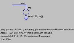
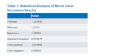
Figure 1 shows a voltage reference modeled in LTspice with a Monte Carlo distribution. The voltage source is nominally 1.25 V, and the tolerance is 1.5%. The Monte Carlo distribution defines 251 voltage states within the 1.5% tolerance range. Figure 2 shows the histogram of the 251 values with 50 bins. Table 1 illustrates the associated statistics of the distribution.

Gaussian Distribution
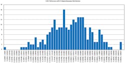
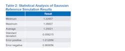
Figure 3 illustrates a voltage reference modeled in LTspice with a Gaussian distribution. The voltage source is nominally 1.25 V, and the tolerance is 1.5%. The Monte Carlo distribution defines 251 voltage states within the 1.5% tolerance range. Figure 4 shows the histogram of the 251 values with 50 bins. Table 2 illustrates the associated statistics of the distribution.
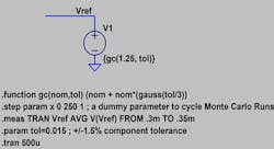
Gaussian distributions are normal distributions with a bell-shaped curve and the probability density shown in Figure 5.

Table 3 shows the correlation between ideal and LTspice simulated Gaussian distributions.

To summarize the above simulations, LTspice can be used to simulate a Gaussian or Monte Carlo tolerance distribution for a voltage source. This voltage source can be used to model a reference in a dc-dc converter. The LTspice Gaussian distribution simulation matches closely with the predicted probability density distribution.
Tolerance Analysis for DC-DC Converter Simulation
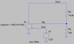
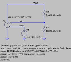
Figure 6 is an LTspice simulation schematic for a dc-dc converter using a voltage-controlled voltage source to model closed-loop voltage feedback. The feedback resistors R2 and R3 are nominally 16.4 kΩ and 10 kΩ. The internal voltage reference is nominally 1.25 V. In this circuit, the nominal regulated voltage (VOUT) or setpoint is 3.3 V.
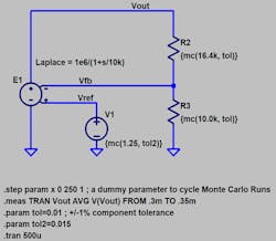
To simulate the tolerance analysis of voltage regulation, feedback resistors R2 and R3 are defined with a tolerance of 1%, and the internal voltage reference is defined with a tolerance of 1.5%. Three methods for tolerance analysis will be presented in this section: statistical analysis using a Monte Carlo distribution, statistical analysis using a Gaussian distribution, and a worst-case analysis.
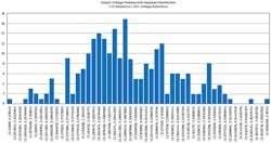
Figures 7 and 8 illustrate the schematic and voltage regulation histogram, respectively, for a simulation using Monte Carlo distributions.

Figures 9 and 10 illustrate the schematic and voltage regulation histogram for a simulation using Gaussian distributions.
Figures 11 and 12 show the schematic and voltage regulation histogram for a simulation using WCA.
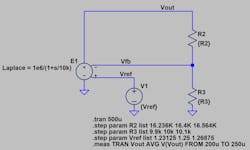
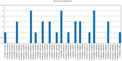
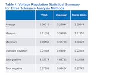
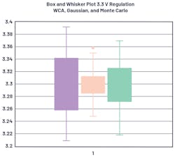
Table 4 and Figure 13 compare the tolerance analysis results. In this example, WCA predicts the largest max deviation, and the simulation based on a Gaussian distribution predicts the smallest. This is illustrated in Figure 13 in a box and whisker plot—the solid box represents the 1-sigma limit, while the whisker represents the minimum and maximum values.
Summary
Using a simplified dc-dc converter model, three variables have been analyzed—two feedback resistors and the internal voltage reference were used to model voltage setpoint regulation. Applying statistical analysis, the resulting voltage setpoint distribution is presented. The results are graphically plotted. This is compared to a worst-case calculation. The resulting data illustrates that worst-case limits are statistically improbable.
Acknowledgements
Simulations were conducted in LTspice, and graphs and plotting were conducted in Excel. The author wishes to thank several anonymous contributors within Analog Devices, and David Rick from Hach, for guidance and insights on this article.
Appendix A
Appendix A is an introduction to the statistical distribution of trimmed voltage references in integrated circuits.
Internal references are Gaussian before being trimmed and Monte Carlo after trimming. The trimming process is typically as follows:
- Measure pre-trim value. The distribution is typically Gaussian.
- Can this unit be trimmed? If not, discard the unit. This step essentially cuts off the tails of the Gaussian distribution.
- Trim the value. This shifts the reference voltage as close as possible to the ideal. Values that are furthest from the ideal are shifted the most. The trimming resolution is only so fine, though, so reference values that are close to the ideal aren’t shifted.
- Measure the post-trim value and lock it if it’s OK.
The resulting distribution has some values unchanged from their original Gaussian distribution, while others are piled up as close as they can get to the ideal. The resulting histogram resembles a column with a dome on top as illustrated in Figure 14.

While this looks more like a random distribution, it’s not. If the product is post-package trimmed, the distribution at room temperature will look like Figure 14. If the product is trimmed at wafer sort, assembly into a plastic package causes the above distribution to spread out again. The result is typically a skewed Gaussian.
Appendix B
Appendix B is a short review of the Gaussian distribution command provided in LTspice. There will be a review of sigma = 0.00333 and sigma = 0.002 distributions as well as some numerical comparisons between ideal and simulated Gaussian distributions. The intent of this appendix is to provide a graphical display and numerical analysis of the simulation results.
Figure 15 is a schematic for a 1001-point Gaussian distribution for the resistor R1.
Of interest is the modification to the .function statement to define the Gaussian function with tol/5. This results in the standard deviation to be 0.002, or 1/5 of the 1% tolerance. The histogram is plotted in Figure 16.
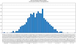
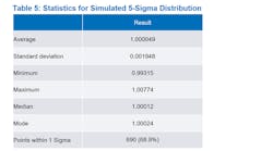
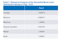
Table 5 shows the statistical analysis of the 1001-point simulation. Of interest is the standard deviation of 0.001948 compared to the expected 0.002.
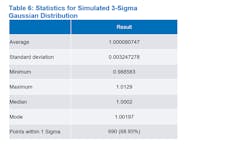
Similar results are presented in Figure 17 and Table 6 for sigma = 0.00333 or 1/3 of the tolerance defined as 1%.

Appendix C
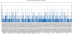
Figures 18 through 21, along with Table 7, represent a schematic for a 1001-point Monte Carlo simulation.


Appendix D
Appendix D reviews how to:
- Edit the LTspice schematic to enable the tolerance analysis.
- Use the .measure command and the Spice Error Log.
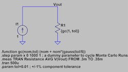
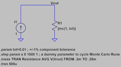
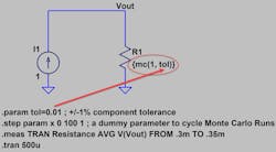
Figure 22 is the schematic for the Monte Carlo tolerance analysis. The red arrow indicates that the tolerance for the component is defined in the .param statement. The .param statement is a Spice directive.
The resistance value of R1 can be edited by right-clicking on the component (Fig. 23).

Entering {mc(1, tol)} defines the resistance value to be nominally 1 with a Monte Carlo distribution defined by the parameter tol. The parameter tol is defined as a Spice directive.
Entering the Spice directive in Figure 22 can be done using the Spice Directive tile on the control bar (Fig. 24).

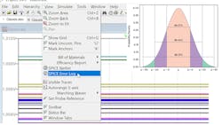
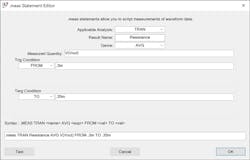
The .meas command has a very helpful GUI for entering the parameters of interest (Fig. 25). To access this GUI, enter the Spice directive as a .meas command. Right click on the .meas command and the GUI will pop up.
The measured data is recorded in the Spice Error Log. Figures 26 and 27 illustrate how to access the Spice Error Log. This also can be accessed directly from the schematic by right-clicking on the schematic as shown in Figure 27.
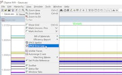

Opening the Spice Error Log presents the measured values as shown in Figure 28. These can be copied and pasted into Excel for numerical and graphical analysis.

About the Author
Steve Knudtsen
Field Applications Engineer, Analog Devices
Steve Knudtsen is a senior staff field applications engineer working for Analog Devices based in Colorado. He graduated from Colorado State University with a BSEE and has been with Linear Technology and Analog Devices since 2000.
Comment About the Article
To join the conversation, and become an exclusive member of Electronic Design, create an account today!

Leaders relevant to this article: