Can EIS Measure Self-Discharge of a Lithium-Ion Battery Cell?

What you'll learn:

• The traditional self-discharge measurement method: delta-OCV.
• A new method for self-discharge measurement: electrochemical impedance spectroscopy (EIS).
• A purpose-built measurement method: self-discharge analyzer (SDA).
• Comparing EIS vs. SDA.

Self-discharge is a normally occurring phenomenon in lithium-ion battery cells.  A normal cell may have a self-discharge rate of 1% state of charge (SOC) per month. The normal self-discharge rate is determined by the temperature of the cell, the SOC, and the electrode materials, while excessive self-discharge is indicative of a faulty cell.  

This fault could be due to issues with the electrode or electrolyte materials, undesirable metal particles contaminating the cells, problems with the separator, or the growth of dendrites. Such faults can be induced poor control of the manufacturing process, by over-charging or over-discharging the cell, or by excessive heating. Click here to view an interesting story regarding an unexpected root cause of self-discharge.

To achieve a high-quality manufacturing process with high yield, factory operators will screen out cells with excessive self-discharge. In addition to checking for self-discharge, other cell performance parameters, like capacity and internal resistance, will be measured and used as part of a complete set of criteria to judge good versus bad.

The Traditional Method: delta-OCV

The common method for self-discharge measurements is called the delta-OCV method. This technique measures the cell’s OCV using a voltmeter; then the cell is placed in constant temperature storage, also known as aging, for three to five days during which the cell will self-discharge. 

The self-discharge will cause a drop in the SOC% of the cell, which results in a lower OCV.  At the end of the storage period, or aging period, the cell’s OCV is measured again. The difference between the first OCV measurement (entering aging) and second OCV (exiting aging) will be a drop of a few millivolts.

A typical delta-OCV is 5 mV, so this could be the threshold amount to determine good versus bad. A cell with a delta-OCV of greater than 5 mV means it has a lower-than-expected SOC% when exiting aging. That’s because it has discharged more than desired during aging due to excessive self-discharge.

Figure 1 is a simple cell model that illustrates self-discharge in the cell. Since the cell isn’t connected to anything, no current can flow into or out of the cell’s external terminals. Therefore, the SOC of the cell isn’t changed through the external terminals. Instead, a current path inside of the cell goes through the internal resistor R_sd. R_sd causes the internal current flow that discharges C_int.

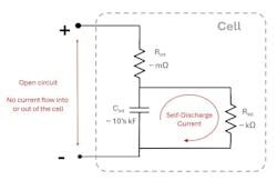
Note that in this model, the component that stored the energy is modeled as an extremely large capacitor C_int with tens or even hundreds of kilofarads of capacitance.  As the stored energy in C_int is removed through resistor R_sd, the voltage across C_int drops, and the OCV drops. Thus, the delta-OCV method measures the OCV change caused by the self-discharging of C_int by R_sd .

While the delta-OCV method is simple to perform, it suffers from the need to store the cells. In a high-volume manufacturing process, storing cells for five days means that there must be a large amount of storage space and high inventory carrying costs. So, the need arises for a better method that can make a good versus bad determination in a much shorter time than three to five days.

Advances in test technology have led manufacturing process engineers to consider two potential solutions for measuring a fast self-discharge:  

1. Measurement and interpretation of the impedance spectrum collected with a spectroscope that performs electrochemical impedance spectroscopy (EIS). These EIS instruments are sometimes called potentiostats.
2. Direct measurement of self-discharge using a specialized instrument called a self-discharge analyzer.

New Candidate Method: EIS

An EIS instrument works by applying a sinusoidal ac current to the cell and then measuring the ac voltage response of the cell. The ratio of voltage to current is resistance R, if measured at DC. However, when an ac current is applied, this measurement is impedance Z. The ac current is swept, and the voltage response is measured at each frequency in the sweep.  Note that the sweep is often stepped over a wide range of frequencies, such a 0.1 Hz to 10 kHz. 

Sometimes, a more efficient method is employed that just checks at a few specific frequencies, which simplifies the EIS instrument, lowering its cost and speeding upthe  time it takes to perform the EIS measurement sweep. Another variation on EIS is to apply a current pulse and use mathematics, such as a fast Fourier transform (FFT), to extract the frequency content of the response of the cell.   

Regardless of which EIS stimulus scheme is used, the fundamental concept is the same:  Apply a range of frequencies of current to the cell and measure the voltage response of the cell at each frequency.

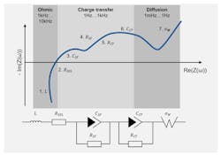
Once the stimulus is applied and the response captured, a chart known as a Nyquist plot is generated by plotting the real impedance on the horizontal axis and the inverse of the imaginary impedance on the vertical axis (Fig. 2, top). The software that controls the EIS will generate the Nyquist plot from the raw sweep data. The Nyquist plot is a common way to represent the electrochemical impedance.

Explaining how to interpret a Nyquist plot is beyond the scope of this article, but fundamentally, the shape of the Nyquist plot reveals characteristics of the cell. Click here for a white paper that delves into EIS for battery testing. 

The physical processes are distributed at different frequencies:

• Inductance of wires and cell structure (at high frequencies).
• Double-layer charging at mid frequencies (100 Hz) is followed by the resistive charge-transfer process at lower frequency (1-100 Hz).
• At low frequencies (<1 Hz), the materials diffusion processes at the electrode are observed.

The EIS data and the Nyquist plot can be further manipulated using equivalent circuit modeling to extract an electrical equivalent circuit model (ECM) of the cell (Fig. 2, bottom).  This ECM will show specific features in the cell, such as the cell’s internal resistance. Click here for an example of software to create an ECM from EIS data.

Purpose Built-Method: Self-Discharge Analyzer

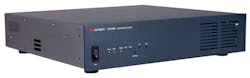
Another way to measure self-discharge is to use a specialized instrument called a self-discharge analyzer (SDA), which is designed specifically for the single task of measuring self-discharge (Fig. 3). The SDA basically micro-recharges the cell as the cell self-discharges, thus preventing cell self-discharge.

While the SDA is making a measurement, it supplies sufficient current into the cell’s external terminals to hold the cell OCV constant (i.e., potentiostatic). The SDA directly measures the required current that it’s supplying, which is precisely the self-discharge current flowing through R_sd in the cell model of Figure 1. Using this method, a self-discharge measurement can be made in as little at 15 minutes.

Comparing EIS to SDA for Self-Discharge Measurement

EIS can be used to learn a great deal about the processes inside the cell (like charge transfer and double-layer charging). It can be manipulated via ECM software to create an equivalent circuit that describes specific elements inside the cell.

However, the self-discharge resistor R_sd can’t be identified using typical EIS techniques. Here’s why: Recall that EIS applies a stimulus frequency (current) that causes a response from the cell (voltage). Effectively, the stimulus frequency causes the relevant processes in the cell to resonate at that frequency. That’s why the equivalent circuit model is often composed of a series of RC circuits, which are also known as resonant or tank circuits, where each RC circuit will be stimulated at a specific frequency.  

In the case of self-discharge, the self-discharge process takes many days to become detectable. For EIS to measure self-discharge and then create an equivalent circuit model that shows the R_sd, the stimulus frequency would need to be extremely slow.

Conceptually, for EIS to measure a a self-discharge behavior that’s five days (432,000 seconds) in duration, the stimulus signal would need to have a period of 432,000 seconds or a frequency of 2.3 μHz. This is an impractical measurement to make.

Alternatively, an SDA can make this measurement in as little as 15 minutes, so this is a practical way to measure cell self-discharge.

While EIS isn’t a good option for self-discharge measurement, it’s a great tool for understanding what’s happening inside a cell. With EIS variants that can quickly and efficiently measure the cell’s impedance spectrum, and with AI/ML software to interpret the results, EIS is suitable for fast determination of good versus bad cells in manufacturing.

But if one of the decision criteria is self-discharge current, EIS can’t be solely deployed. Instead, the manufacturing test process must include both SDA and EIS.