Triggering morphs to match application needs
When Tektronix introduced Howard Vollum’s Model 511 triggered-sweep oscilloscope in 1946, it was a game-changer. Triggering allowed users to isolate critical parts of a waveform, which facilitated faster and more comprehensive circuit troubleshooting. During the next 71 years, triggering would be extended to multiple domains and types of signals, increased in speed and sensitivity, and implemented digitally.
Higher speed triggering has followed improvements in semiconductor technologies, changing first from discrete circuitry to ICs, then to silicon ASICs, and finally to full-custom implementations using the latest materials and processes. The signal characteristics that can be recognized as trigger events also have evolved, today including several serial bus protocols as well as a wide selection of lower-level time and voltage combinations.
Whether triggering is hardware- or software-based is yet another factor that makes a big difference. To handle high-bandwidth signals, many companies have expanded the types of trigger events handled by hardware. As Melissa Spencer, Infiniium product brand manager at Keysight Technologies, said, the company’s S-Series scopes feature a long list of hardware-supported trigger types including those related to edges, pulses, patterns, windows, and even some serial-bus protocols. In addition, you can choose to put any two hardware trigger events in series so that one condition must be satisfied before the other.
Spencer further explained, “Software triggers are used on Infiniium oscilloscopes when the trigger condition is more complex than what the hardware can handle alone. First the oscilloscopes trigger in hardware to acquire the waveform data. Then event searching happens in software…. Because software triggering occurs after hardware trigger, acquisition, and analysis of the acquisition, software triggering is slower than hardware trigger.” The S-Series scopes use software to trigger on the results of measurements, a
user-defined serial protocol condition, runt pulses, and nonmonotonic edges. In addition, you can set up and logically combine as many as eight zones to define complex trigger events.
Several oscilloscope design trends are related to triggering. For example, a high waveform update rate can be beneficial when looking for the source of an infrequently occurring fault. Many manufacturers have developed color-graded persistence displays that help to highlight waveform anomalies.
Another trend is to provide large acquisition memories—often several megabytes. Users should be aware that long acquisition records and fast update rates are mutually exclusive. The Rohde & Schwarz Model RTE with a standard 10-MB memory length per channel provides a good example of the trade-offs involved. This instrument samples at a maximum 5-GS/s rate and claims up to 1-M updates/s. The greatest memory length that can be used to achieve this update rate is 5,000 samples. Of course, the signal source must satisfy your selected trigger condition sufficiently often that it’s possible to achieve the desired
update rate.
And some companies have developed special acquisition modes to support high update rates. For example, to have the highest rate offered by many Tek scopes, you must use the FastAcq mode, which builds a pixel map by overlaying successive short acquisitions. The intensity or color of each pixel corresponds to the number of times that waveforms crossed through that point. FastAcq, as it has been implemented in some Tek scopes, is based on 500-sample acquisitions and achieves at least 400 k updates/s.
Trigger jitter
Precisely positioning the displayed trace relative to the trigger point is a topic that continues to attract interest. Many older DSOs simply didn’t address the problem. Nevertheless, trigger jitter didn’t necessarily cause discernable measurement error. Early DSOs that used conventional CRTs displayed from 1,000 to 4,000 points along the horizontal axis. Generally, the CRT spot size was large enough that you couldn’t tell the difference between a signal that was synchronous with respect to the sampling clock and one that wasn’t. This was not the case if trace magnification was used, which spread out the spacing between samples and resulted in a blurred trace if the trigger position jittered.
One way the problem could be solved was to note the time delay between the actual triggering instant and the next sample point. By delaying the trace DAC output relative to the start of sweep, better trace-to-trace alignment could be achieved. Alternatively, because trigger jitter is caused by variations in the time difference between the triggering instant and the free-running time-base clock, attempts were made to match the time-base phase to the trigger timing.
Approaches of this type come under the startable oscillator heading. Several patents have been filed that describe oscillators in which the phase can be instantaneously altered in response to a control signal, such as the output from a trigger circuit.
The situation significantly changes when a flat panel with fixed pixel locations is used as the display device. To eliminate the effects of trigger jitter in successively displayed traces, the jitter must be removed from the trace data before it’s displayed. This is where interpolation comes in.
Interpolation
If you can determine what the original analog signal looked like between sampling instants, then you can subdivide a sampling period to achieve greater timing resolution. Some scopes claim to have very high direct-sampling time-base speeds, but the highest displayed rates often are just expanded versions of the maximum hardware sample rate. In this case, interpolation between actual samples allows a detailed view of the (reconstructed) waveform.
In both this case and when a hardware-supported time-base speed is selected without expansion, interpolation can be used to reduce the effect of trigger jitter. For example, if you assume that the resolution of the trigger-to-sample timer is 100 ps and the highest hardware-supported sampling rate is 1 GS/s, then interpolation needs to subdivide a sampling period into 10 segments. Successive traces will display the minimum trigger jitter if in each displayed frame the interpolated trace data is offset from the true sample positions by the number of subdivisions corresponding to the trigger-to-clock delay for that frame.
Interpolation has wide application but also a few restrictions. According to Shannon, a band-limited signal x(t) that has been sampled at greater than twice the highest frequency component can be reconstructed by applying the equation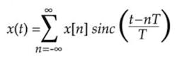
An appropriately scaled sinc function equals zero at all non-zero integer arguments and equals the value of the nth sample at t = nT—in other words, the reconstructed waveform will exactly equal the value of successive samples at the sampling instants. However, the importance of the process lies in its capability to accurately determine all the unknown values between successive samples.
Today, an instrument designer might implement a lookup table with precalculated and scaled sinc values or use a DSP-based interpolating filter to upsample the original data points. Trigger jitter is minimized by displaying a new set of samples offset from the original data samples by the trigger-to-sample delay for each acquisition.
In the early 1980s, using these techniques was impractical and advanced components didn’t exist, which made developing a product such as the two-channel Gould Biomation 4500 100-MS/s DSO a bold undertaking. Even ensuring that circuits based on the available ECL ICs would reliably function at 100 MHz took some effort—to minimize circuitry and reduce propagation delays, the instrument featured a 1-2-4 time-base speed relationship rather than the more conventional 1-2-5 sequence. Also, the 1,000-point acquisition memories each consisted of two ping-ponged banks because IC memory access time exceeded 10 ns.
In 1981, the company’s William Shoemaker addressed the problem of interpolation with an approach described in U.S. Patent 4,455,613, “Technique of reconstructing and displaying an analog waveform from a small number of magnitude samples.” The Intel PL/M-86 compiler code listed in Appendix II of the patent is labeled “4500 Sine Interpolation Procedures”—4500 users could select “linear” or sine interpolation.
As described in the patent abstract, “…The analog waveform slope at each sample is calculated from the magnitude of the two samples taken from the waveform immediately preceding a given sample and the two immediately following the given sample. A slope of the analog waveform intermediate of each sample interval is then calculated from this information, leading to a final calculation of the magnitude of a selected series of points during the sample interval.” This is an approximate algebraic method in contrast to a more rigorous approach that might use an interpolating filter or transcendental functions and as such was practical to implement on a microprocessor available at that time.
Digital triggering
One of the earliest uses of the term “digital trigger” is in the 1983 Hewlett-Packard catalog where the 5180A dual-channel 20-MSa/s digitizer is described as using digital triggering. Although digital trigger seems generic, it isn’t. It specifically refers to the use of the digitized data from a channel’s ADC as the trigger signal. This very narrow meaning has been continued by National Instruments, Rohde & Schwarz, Pico Technology, Siglent Technologies, and Rigol Technologies—NI, Siglent, and Rigol for only some of their products, Pico and R&S for all of them. Digital triggering should not be confused with pattern or state triggering, generic terms used by virtually all manufacturers whether or not their instruments use digital triggering.
Why digital? According to NI’s Ben Robinson, product marketing manager for modular instruments, it’s to achieve greater accuracy, “… by avoiding a trigger circuit that is made up of analog components separate of the main ADC signal path…. [And] … digital triggers allow for interpolation methods that can deliver sub-sample trigger resolution, like the PXIe-5164 oscilloscope interpolator which yields 1-ps resolution.” R&S claims similar advantages and includes a highly expanded trace display in the company’s literature to demonstrate the low trigger jitter that has been achieved. Figure 1, a block diagram representing the NI PXIe-5170R reconfigurable multichannel DSO, shows ADC outputs directly connected to the scope’s FPGA to facilitate digital triggering.
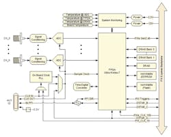
Courtesy of National Instruments
Teledyne LeCroy’s Christopher Busso, product line manager, noted that digital triggering can create errors if the sampling rate is too low relative to the signal bandwidth: “If you’re not sufficiently oversampling the input signal, triggering can be inaccurate.” He continued, “On the positive side, most front-end amplifiers have two outputs: one feeds the ADC while the other feeds the triggering chip. This means that despite the best efforts of oscilloscope design teams to match impedances, path lengths, and pay attention to things such as thermal tails, the reality is that the ADC and triggering chip see different signals. However, with digital triggering, it’s a single path: The signal is digitized and then triggered, so those differences in signal are eliminated. The oscilloscope is triggering on what you see on screen vs. seeing one thing and triggering on something else.”
Pico Technology’s Kieran Winstanley, distribution sales manager at the company, commented, “With digital triggering, … the displayed waveform is always synchronized with the trigger point on the screen, so horizontal jitter is never more than one sample period and the waveform appears stable. PicoScope oscilloscopes improve on this by using a calculation technique to reduce the displayed jitter to a small fraction of a sample period.”
A further benefit is improved sensitivity. Because the same ADC data that is acquired also is used for triggering, trigger sensitivity is determined by a channel’s input attenuator/preamplifier combination. Winstanley continued, “On the vertical axis, digital triggering guarantees that the trigger threshold voltage is stable and accurate to within one LSB of the ADC’s output range. On an 8-bit scope, this gives a precision better than 0.4%” This is in contrast to most analog trigger specifications that typically require much larger excursions for very fast pulses or high frequencies.
Siglent’s Steve Barfield, general manager, said that digital triggering is used in the SDS2000X/SDS2000, SDS1000X/SDS1000+, and SDS1000X-E models. According to information on the company’s website, “[The SDS2000X] has an innovative digital trigger system with high sensitivity and low jitter and a maximum waveform capture rate of 140,000 wfm/s (normal mode), up to 500,000 wfm/s (sequence mode). It also employs the common 256-level intensity grading display function but also a color temperature display mode. The trigger system supports multiple powerful triggering modes including serial bus triggering.”
Rich Markley, oscilloscope product manager at R&S, agreed that digital triggering has many pros but there is an important con especially for high-bandwidth designs. He said, “The biggest drawback is in the design complexity. [In the RTO,] because we are analyzing all ADC samples in real time, we must be able to process 80 Gb/s of data (ADC runs at 10 GS/s @ 8-bits), not a trivial task.”
Analog Triggering
Another clue to the practicality of analog triggering was given by Rigol’s Chris Armstrong, director of product marketing and SW applications, who said, “Rigol uses a mix of [analog and digital] capabilities to maximize effectiveness. The 1000Z Series scopes, which are lower speed, utilize digital triggering for clarity and convenience of captured signals, while our [faster] scopes like the 4000 series trigger on analog [signals] for higher performance and more specific trigger requirements.”
Nevertheless, according to Markley, “In analog trigger systems, [trigger jitter] is typically addressed via software correction, which slows the oscilloscope.” Still, this may be a reasonable trade-off. Tek’s David Njuguna, technical marketing manager, described the sub-40-ps glitch-width analog trigger capability of the company’s 70-GHz-bandwidth DPO70000SX Series oscilloscope. Of course, there is a relationship between glitch width and the required amplitude, but the trigger circuit reliably identifies a point on the glitch with much less than 40-ps uncertainty.
Main channels on the DPO70000SX sample at up to 200 GS/s—20x faster than the R&S scope to which Markley was referring when citing the 80-Gb/s data processing rate. In comparison, performing real-time analysis at 1,600 Gb/s seems unrealistic—at some speed, digital triggering becomes impractical.
Siglent’s change from analog triggering on the earlier SDS1000 instruments to digital triggering on the later SDS2000 Series appears to be performance related. Both series sample at a maximum 2-GS/s rate, so digital triggering can be implemented by an FPGA-based design. The company’s Barfield commented, “In the analog triggering system, the trigger path acts as a stub on the analog signal path, which introduces more parasitic parameters and reflection. In the digital triggering system, the trigger path is in the FPGA, so signal distortion on the analog signal is minimized.”
It should be noted that Shannon was not concerned about scope triggering. In addition to band limiting, the only other requirement for perfect reconstruction is the use of a constant sampling frequency. So, although there is a timing accuracy advantage to a digital trigger system, interpolation is equally practical for scopes that use analog triggering.
Recent advances
Improved protocol triggering is an area addressed by several manufacturers. As explained by Tek’s Njuguna, the high-speed serial link training analysis (HSSLTA) option for the company’s DPO70000SX scopes, “… uses the power of DPO70000SX triggering to identify link training exchanges between devices, then analyzes and displays the protocol, timing, and PHY signaling associated with negotiation of 100 Gb/s links. This insight allows designers to verify the link training process and to quickly pinpoint problems when the links fail to train.”
Also highlighting protocol triggering and decoding, Keysight has expanded the range of available options for the Infiniium Series scopes. ARINC 429 and MIL-STD-1553 (N8842A); USB 3.1 Gen1/Gen2 (N8821A); CAN, LIN, FlexRay and CAN-FD (N8803C); 10BASE-T/100BASE-TX Ethernet (N8825B); and I3C (N8843A) protocol triggering and decode options have recently been introduced.
A very important feature of many improved protocol triggering options is time-correlated cross-domain views. For example, Keysight’s Spencer explained that for the company’s N8821A, “This application has a multitab protocol viewer enabling you to quickly move between the physical and protocol layer information using a time-correlated timing marker.” And, as the company’s website states, “The N8825B 10BASE-T/100BASE-TX Ethernet protocol decoder provides time-correlated views of physical layer (raw data) and transaction layer packets. [The] Unique packet-waveform correlation marker makes it easy to scroll through waveforms to view synchronized packet and symbol lists.”
The R&S RTO2000 features zone triggering in the time and frequency domains—at the same time (Figure 2). The company’s Markley commented that zone triggering was “… especially powerful in the frequency domain as it is sometimes easier to see an issue in the frequency domain versus the time domain. A great example is EMI debug where you might be looking for an offending signal at a specific frequency. By setting the trigger in the frequency domain, you then get a correlated trigger across all signals (analog, protocol, digital, frequency). In addition, our history mode allows the user to go back in time to see previous trigger events.” He concluded, saying that the zone trigger capability “… works beyond just [the] frequency domain to allow triggering on any math function.”
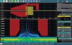
Courtesy of Rohde & Schwarz
In a modern implementation of an old idea, Teledyne LeCroy has developed the HDA 125-18-LBUS mixed-signal test solution (Figure 3). Years ago, before integrated MDOs were popular, pattern or state triggering could be added to DSOs by attaching a logic trigger pod to the external trigger input.
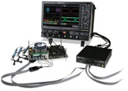
Courtesy of Teledyne LeCroy
The HDA product also is a separate assembly, but as the company’s Busso explained, “Its primary application is acquiring and triggering on up to 18 high-speed parallel digital channels with a sampling rate of 12.5 GS/s. The premier application for HDA 125-18-LBUS is DDR memory. We’ve built specialized DDR command-bus triggers into our DDR Debug toolkit that enable HDA 125-18-LBUS to trigger on specific DDR command-bus requests. Coupled with our QuickLink probing solution that enables seamless transitions from digital to high-bandwidth analog-signal acquisitions, the HDA 125-18-LBUS mixed-signal test solution makes validation of challenging interfaces such as DDR4 both simpler and more comprehensive….”
Although many products emphasize hardware trigger performance, the flexibility provided by software triggering can be an advantage. NI’s Robinson mentioned the NI-TClk software synchronization tool the company provides, which can “… align the triggering and sampling of instruments of many types to achieve trigger jitter of less than 100 ps across all instruments in a single PXI chassis.”
A recent Pico Technology press release announced the addition of CAN FD decoding to the company’s PicoScope 6 software, which “… can already decode a wide variety of serial protocols such as I2C, SPI, and UART, as well as automotive standards such as CAN, LIN, and FlexRay,” said Trevor Smith, business development manager, Test & Measurement. “Now it can also decode CAN FD, which is the latest and fastest version of CAN Bus used in automotive and industrial automation applications.”
And, Rigol’s Armstrong noted that the company continues “… to expand the capabilities of existing instruments…. Last year, we added LIN triggering and decoding to the 4000 Series. This expands on our automotive-focused triggering that already included CAN and Flexray. LIN trigger and decode was immediately added to our free options bundle for all new 4000 Series instruments.”
For More Information
About the Author

Tom Lecklider
Comment About the Article
To join the conversation, and become an exclusive member of Electronic Design, create an account today!

Leaders relevant to this article: