Spice Simulates Custom Random Distributions for Monte Carlo Analysis

Download this article in PDF format.
Not all Spice versions perform Monte Carlo simulations. Even those that do may only have a small number of available distributions, much less custom ones. LTSpice, for example, has built-in random distributions limited to Uniform and Gaussian (defined by sigma, but no specified limit). Unfortunately, this excludes many real-world distributions such as Gaussian (with maximums of 2-sigma, 3-sigma, etc.), bimodal, triangular, and U-shaped for example. A review of web reference shows few solutions beyond the available functions.
However, using straightforward statistical theory, you can create a random process of any distribution listed above. Even histograms from manufacturers’ datasheets or your own lab measurements are easily simulated. What are the minimum requirements? A calculation tool having a uniform random-number generator and a lookup table function. We’ll apply the method here using Excel and Spice.
This statistical/simulation adventure was both fun and insightful. The nuts and bolts of creating a circuit simulation developed an intuitive understanding beyond the abstract statistical theories.
The Method
Four easy steps define what’s called the Inverse Sampling Method. You can apply this with various calculation tools.
- Create a Probability Density Function (PDF) of your desired random distribution by calculating a function or entering the data f(x).
- Calculate the Cumulative Distribution Function (CDF), which is simply a running sum of the PDF, u = F(x) = (-∞ to x) ∑ f(x).
- Find the Inverse CDF (ICDF) by swapping the input and output data, x = F-1(u).
- Use the ICDF as a lookup table with a uniform random number generator (0 to 1) driving the input (CDF) and the output having values of your desired distribution (x).
Here’s a simplified block diagram for the method (Fig. 1).
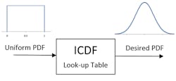
1. The Inverse Sampling Method’s block diagram.
Specific to an Excel/Spice implementation, the method becomes:
- Create a PDF as a function of x in a column of an Excel sheet.
- Calculate the CDF as a running sum of the PDF. Normalize the CDF so that the max value is 1.
- ICDF
- Define the ICDF by identifying the CDF as input and x as the output.
- Create a comma-separated string for the ICDF (VBA code) with ordered pairs of CDF as input and x as the output of a lookup table. Copy string into Spice’s Table function.
- Use Spice’s uniform random function (range 0 to 1) as input to the Table to generate an output x having the PDF of your desired variations.
An RC Filter Example
Let’s jump into a filter example. We’ll estimate the performance variations given the RC component tolerances. But what are their distributions? The resistor has a 1% tolerance with a Gaussian distribution having a standard deviation of 1/3 the maximum tolerance (3-sigma max). To cost-reduce the filter, the capacitor was selected having a 10% tolerance with a Bimodal Gaussian distribution where the center 5% has been removed for higher precision grades.
Step 1: Define the PDF
For the resistor, create a generic 3-sigma max Gaussian distribution with the following parameters: Upper Limit / Lower Limit = 1 / -1, mean μ = 0, sigma σ = 0.33. We can always scale this distribution in the Spice simulation for any tolerance with this shape. A 21-point PDF was chosen. You can use more or less points depending on the complexity of PDF’s shape.
First create a column of x values in Excel from -1 to 1 over 21 points (Fig. 2, top). This column is created on the far right—think lookup table needed later.
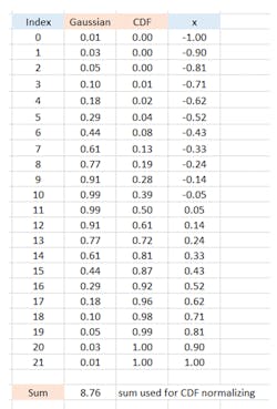
2. Excel’s columns for x, PDF and CDF (top); plots of PDF, CDF, and ICDF for a Gaussian distribution with a 3 Sigma Max limit (bottom).
In another column, calculate the PDF using the equation:
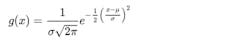
The plot of the PDF appears in Figure 2 (bottom).
Step 2: Calculate the CDF
In the next column, create the CDF by calculating a running sum of the PDF. Normalize the CDF by dividing each value by the total sum of the PDF. (Strictly speaking, the PDF should have area under the curve equal to 1. However, for convenience and to ensure a proper CDF, we’ll normalize here.) The plot of CDF, spanning 0 to 1, shows a nice intuitive shape where the sum accumulates slowly at the Gaussian tails and more rapidly at the Gaussian’s peak at the center (Fig. 2, bottom).
Step 3: Define the ICDF
To find the ICDF, no actions are required! Simply swap axes defining the CDF as input and x as output. The plot of ICDF (Fig. 2, bottom) has an input range of 0 to 1 and an output range of −1 to +1, which is that of our desired PDF. Notice for the Gaussian PDF how most of the output values (vertical axis) fall near the center of the curve as expected. (If you wish to perform Monte Carlo simulations within Excel itself, use the RAND function as the input value to the VLOOKUP function with CDF as input column and x as the output column.)
Step 4: Construct Spice Lookup Table
Now let’s cross boundaries into Spice land. The trick here lies in converting the ICDF into a format of your particular lookup TABLE function. In LTSpice, the table function is defined as
table( input, x0,y0,x1,y1, ... )
which interpolates an “input” based on a lookup table given as a set of “xn,yn” pairs. A simple VBA function was written to create a string in this table format. The function “get_Table(Cell range of CDF, Cell range of x)” is easy to understand and modify (in Excel, hit Alt-F12 to view the code). With basic string manipulation, it returns a text string with ordered pairs of CDF and x. To get a useful text string from the getTable() function, select the cell and copy the “values” into the cell below it.
Table(input ,0,-1,0,-0.9,0.01,-0.81,0.02,-0.71,0.04, … )
Step 5: Generate Random Variable in Spice
Next, copy your Table string into an LTSpice function, named gauss3() in this example.
.function gauss3() Table( uniform(), 0,-1, 0,-0.9,0.01,-0.81, … )
Notice in the Table, you replace the original “input” with “uniform()”, which is another function created for convenience using LTSpice’s built in flat() function.
.function uniform() flat(0.5)+0.5
Resistor Tolerance
Finally, how do you get your random number to vary a component during simulation, say a 10k resistor having a 1% tolerance with a 3-sigma limit? Because LTSpice allows expressions and functions for the component values, you set the resistor value to:
{ 10k* (1+0.01*gauss3()) }
Capacitor Tolerance
The PDF for our filter’s capacitor has an interesting PDF shape referred to as a bi-modal distribution. Although it’s a 10% part (for our budget RC filter), the center 5% values have been removed for higher precision grades.
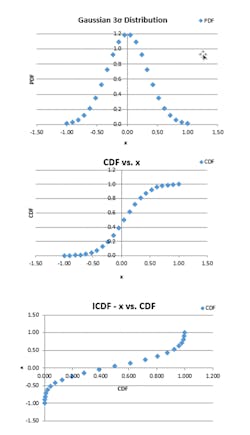
A generic PDF is created in the range of ±1 with a Gaussian (2-sigma max) distribution where the center ±0.5 has been removed. How was this accomplished? A Gaussian equation was used along with an “IF” function to zero out the center values. The plots for this bi-modal distribution reveals an intuitive understanding of the method (Fig. 3). First, the PDF with a Gaussian distribution shows a center with 0 probability.
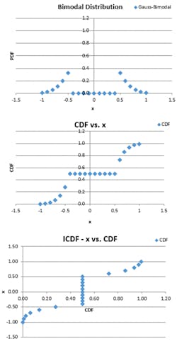
3. Plots of PDF, CDF, and ICDF for a bi-modal distribution.
Next, notice how the CDF goes flat across the center! This is where the PDF’s 0 probability forces the CDF’s running sum to remains constant. Finally, the ICDF shows how the values ±0.5 are being skipped altogether on the output (vertical axis).
Following the same table creation described for the resistor, the LTSpice function looks like:
.function bimodal() Table(uniform(),0,-1,0,-0.9,0.01,-0.81, … )
To create a 1-nF capacitor with 10% max tolerance, set its value to:
{ 1nF * (1+0.10*bimodal()) }
Monte Carlo Spice Simulation
Okay, let’s see it all work together to predict the filter’s variations over 51 runs of a 100-µs time-domain (Transient) simulation. Of particular interest is the rising edge of a fast pulse passed through our filter. The LTSpice schematic is shown in Figure 4.
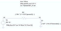
4. LTSpice file with component values and commands for performing Monte Carlo Analysis.
For convenience, the ICDF tables have been saved in a separate text file—please go to http://ecircuitcenter.com/Calc/MC_LTSPICE.html to access the file. The .INC statement let’s Spice know to include this in the simulation. The Step command requests 51 repeated runs of the Transient analysis.
So how does our filter respond to a fast edge over 51 variations of R and C? The plot confirms our expectations (Fig. 5).
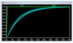
5. LTSpice plot of step response for an RC filter showing effects of the capacitor’s tolerance having a bi-modal distribution.
The rise times are clustered around two values, dominated by the capacitor’s bi-modal distribution. The resistor’s Gaussian variations also contribute to the spread of the rise times. (Note: This is where Monte Carlo analysis can really shine over other analyses, especially for non-Gaussian distributions. The Root-Sum-Squares (RSS) method may overestimate the maximum error, while the Worst Case Analysis method would not predict the variations in a production test. But that’s another design story.
Datasheet Histograms
Is it possible to replicate random distributions from manufacturers’ datasheets or lab data of your own components/subsystems? Say an op amp manufactures publishes a histogram of an unusual distribution for an input offset voltage (Fig. 6).
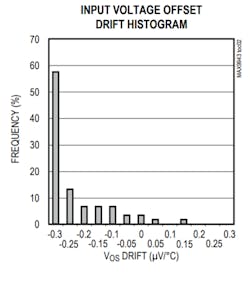
6. Manufacturer’s datasheet showing skewed histogram of input offset voltage drift.
Although you could try fitting an equation to this skewed PDF, simply enter the values from the histogram into the “PDF” column and create an “x” column representing the drift values from −0.3 to +0.3 µV/C. The cell calculations and VBA code deliver your Table function.
.function voffTC1() Table(uniform() , 0,-0.3, 0.53,-0.25, …, 99,0.3)
As a sanity check, let’s run a test simulation (Fig. 7) adding LTSpice’s MEAS function that captures the level at vo over 101 runs in the *.log file.

7. Spice schematic of circuit used to test skewed statistical variations of input offset voltage drift.
Does voff1’s random values resemble anything close to the device’s datasheet? Importing the log file into Excel, we see the histogram (Fig. 8) of 101 tells a story of the distribution for v(vo) correlating well to the datasheet’s histogram.
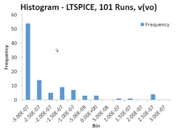
8. The histogram of 101 runs of voltage drift for voff1.
Lab and Production Data
What about the variations of your lab or production data? Simply create a histogram of your data experimenting with the number of bins until the shape of the simulation’s histogram reasonably matches that of your original data. Then turn the crank on the method as demonstrated above.
Conclusion
The Inverse Sampling Method is a powerful method to create random variations of custom PDFs. You can easily apply this method using any calculation tool with a uniform random generator and a lookup table function.
TO ACCESS THE EXCEL AND LTSPICE FILES, GO TO: http://ecircuitcenter.com/Calc/MC_LTSPICE.html.
Rick Faehnrich is Senior Analog Design Engineer at Teradyne Inc.
References
Tolerance Design of Electronic Circuits, Robert Spence, Randeep Singh Soin, World Scientific, 1997.
Inverse Sampling Method, Mathworks, https://www.mathworks.com/help/stats/generate-random-numbers-using-the-uniform-distribution-inversion-method.html.

About the Author
Rick Faehnrich
Senior Analog Design Engineer
Rick Faehnrich designs precision analog circuits for Teradyne Inc. For three decades, he’s developed analog circuits, control systems, and filter algorithms in the ATE, X-ray imaging, medical, and automotive fields. He enjoys bridging the gap between textbook and real-world engineering through training sessions and publishing a website that focuses on Spice for learning analog design (www.ecircuitcenter.com).
Comment About the Article
To join the conversation, and become an exclusive member of Electronic Design, create an account today!

Leaders relevant to this article: