The Chronicles of GND (Part 4): Supply Currents—When Simulations are Both Correct and Wrong

I was going to take a break from “The Chronicles of GND.” But “Push Me, Pull Me” resulted in a surge of correspondence—much of it criticism that I had not included any diagrams of the various forms of current flow in the output stages I described in that post. I was telling, not showing—a cardinal sin for a wannabe storyteller.
So, the first thing I intend with this post is to include diagrams to illustrate the story that I’d like to tell. Gather round; like so many good stories, this is a cautionary tale. It’s not about single-supply circuits or the mysteries of GND per se. But supply current does play the “canary in the coal mine” role here.
This is principally a story about being misled by simulation. The much-missed Bob Pease was well-known to be deeply distrustful of it. I must confess to being rather more of a fan of simulation, but I’m in agreement about the pernicious ease with which we engineers can treat the results of a Spice simulation as “correct.”
The roots of the tale lie in the discipline of inductive proximity sensing, which has been engaging some of my colleagues recently. In its simplest form, a coil “sniffs” its electromagnetic environment. The coil is “tuned” with a shunt capacitor, to form a resonant (“tank”) circuit, and that circuit is driven with a high-ish frequency signal. Figure 1 shows the basics.
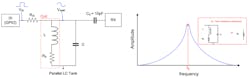
1. The basics of fixed-frequency eddy-current proximity sensing.
The presence of a conductive target that can support the flow of an induced eddy current affects the properties of the coil. Typically, the inductance falls and the loss increases as the target approaches the sense coil. The combination of the sense coil and the target behaves like a low-quality transformer, with a secondary made from a single shorted turn that’s poorly, and variably, coupled to the primary. It’s simple to model this in SPICE.
When I got involved, I looked at the circuit, and pretty much the first comment I had was, “Well, you’ll need a capacitor in series with the drive to eliminate the static DC current drain through the coil.”
The essence of my colleagues’ rebuttal to this was along the lines of: “We’re driving that tank circuit near resonance. At resonance, the impedance is pretty high, so the power dissipated is pretty small. Nothing to worry about.”
“Ah,” I replied, “but you are driving the tank with a signal that’s the sum of a pure AC signal—which doesn’t dissipate much in the resistive loss of the tank, sure—and a DC pedestal of around half the supply voltage. This causes a static current to flow in the series combination of Rdrive and Rser there.”
They weren’t convinced, so they decided that this case should be tried in a court of simulation. A young engineer was duly assigned to craft the necessary simulation model and determine the truth of the matter. This suited me fine. He’d simulate with and without the blocking capacitor, I’d be proven right, and my reputation as a Filter Wizard would be secure. Job done, no effort on my part. Imagine my surprise…
“The capacitor makes no difference. Simulation proves it. Kendall’s wrong.” Well, the engineer didn’t say the last bit, but I knew everyone was thinking it. And I realized, in some small way, what it was like to be Bob Pease because my first thought was, “Well, if the simulation says that the capacitor makes no difference, then the simulation is wrong.”
I built my own simulation schematic for the test circuit, incorporating two complete instances differing only by the inclusion or not of a suitable DC blocking capacitor. I used bona fide values for the circuit parameters, to match a particular configuration. Figure 2 is a screenshot from LTspice.
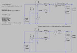
2. Comparing tank driving circuits with and without a DC blocking capacitor.
You’ll notice that instead of just driving the tank with a source of some kind, I built a little output stage with pull-up and pull-down switches. This enables me to check on the current being drawn from the supply (and also being injected into GND). I used an expression to make it easy to drive the tank at its resonant frequency (which isn’t always the right thing to do, but that’s not germane here).
When all seemed ready, I clicked LTspice’s tiny running-man icon, then watched as the supply currents in the pull-up and pull-down devices of the I/O pin driving the circuit appeared on screen…
… essentially the same for both instances (Fig. 3). The same with or without that 100-nF coupling capacitor. After a short period of stabilization due to the inherent Q factor of the tank, both plots produced a stable plot with the shape I expected. And the DC blocking capacitor appeared to have no significant effect. My head was spinning. It does not compute…
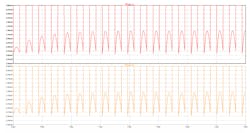
3. Supply current taken by the two configurations, just after switch-on.
But, there was a small difference building up at the end of the 4-µs analysis period. What happens if you extend the analysis period… and then it clicked. The DC blocking capacitor introduces an extra time constant into the circuit; after switch-on, the capacitor has to charge up to its steady-state voltage through a series resistance of around 1 kΩ. With 100 nF, that’s a time constant of 100 µs right there. So, let’s look at the comparison if we wait for long enough (Fig. 4).
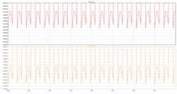
4. Supply current taken by the two configurations, after waiting 100 µs.
Bingo! Now, when steady state is achieved, the DC blocking capacitor is doing its job, and there’s no static current component flowing in the coil. And, as I had gut-felt right at the start, this reduces the overall peak and average current being drawn from the supply—something that practically every customer is concerned about.
Using the current monitor in LTspice, I could easily check the currents for the two cases. Figure 5 shows the currents for the case without the blocking cap. Figure 3 showed the version with the blocking cap looking essentially identical, but we now see the upper current trace in Figure 4 showing substantially smaller currents—confirmed by the currents shown in Figure 6.
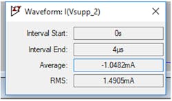
5. Average current when no DC blocking cap is present.
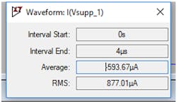
6. Average current when a DC blocking cap is used.
It’s instructive to play with the value of that DC blocking capacitor. It turns out that it doesn’t need to be nearly as large as the use-everywhere “point one,” the 100 nF. Something like 20 times the tank resonating capacitor is fine. If we had done the simulations with a much lower value for this capacitor, we would have seen the difference building up straight away… and I would never have had the chance to pass this message on.
What’s the moral of this story? Keep your eyes peeled for all of the time constants in the circuit you’re looking at. Remember that when you click that start button on your simulator, your circuit starts simulating from time t=0. Before that time, the circuit wasn’t operational, and conditions in the network may well not yet represent the steady state.
The simulator is giving you the correct answer to the wrong question. When we run a simulation, we only see the answer (which it gives us) and not the question (which we coded into the simulation, sometimes without enough thought). So it’s easy to assume that the simulation is answering the question in our heads, not the question represented by the simulation. And perhaps that’s what frustrated Bob so very much. Drop me a line if you’ve got a similar (or should that be simular) tale!

About the Author
Kendall Castor-Perry
Senior MTS Architect, Programmable Systems Division
For nearly four decades, Kendall Castor-Perry has been chasing signals through electronic systems, wringing out the information they are hiding. He’s a world-class authority on filters and precision analog circuit engineering and a tireless champion of the needs of the customer. He has been widely published and syndicated, especially when sharing his extensive filtering knowledge as “The Filter Wizard.” He holds a BA in Physics from Oxford and an MBA in MBA stuff from London Business School. Kendall is currently Senior MTS Architect in Cypress Semiconductor’s Programmable Systems Division, pushing on the performance:power:price boundaries constraining tomorrow’s critical sensor-processing systems.
Comment About the Article
To join the conversation, and become an exclusive member of Electronic Design, create an account today!

Leaders relevant to this article: