Back to Basics: Impedance Matching (Part 1)

This article is part of the Analog Series: Back to Basics: Impedance Matching

The term “impedance matching” is rather straightforward. It’s simply defined as the process of making one impedance look like another. Frequently, it becomes necessary to match a load impedance to the source or internal impedance of a driving source.
A wide variety of components and circuits can be used for impedance matching. This series summarizes the most common impedance-matching techniques.
Rationale And Concept
The maximum power-transfer theorem says that to transfer the maximum amount of power from a source to a load, the load impedance should match the source impedance. In the basic circuit, a source may be dc or ac, and its internal resistance (Ri) or generator output impedance (Zg) drives a load resistance (RL) or impedance (ZL) (Fig. 1):
RL = Ri or ZL = Zg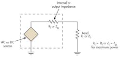
A plot of load power versus load resistance reveals that matching load and source impedances will achieve maximum power (Fig. 2).
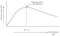
A key factor of this theorem is that when the load matches the source, the amount of power delivered to the load is the same as the power dissipated in the source. Therefore, transfer of maximum power is only 50% efficient.
The source must be able to dissipate this power. To deliver maximum power to the load, the generator has to develop twice the desired output power.
Applications
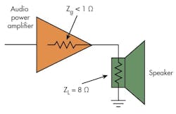
Delivery of maximum power from a source to a load occurs frequently in electronic design. One example is when the speaker in an audio system receives a signal from a power amplifier (Fig. 3). Maximum power is delivered when the speaker impedance matches the output impedance of the power amplifier. While this is theoretically correct, it turns out that the best arrangement is for the power amplifier impedance to be less than the speaker impedance. The reason for this is the complex nature of the speaker as a load and its mechanical response.
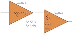
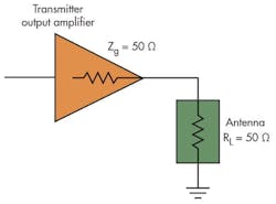
Another example involves power transfer from one stage to another in a transmitter (Fig. 4). The complex (R ± jX) input impedance of amplifier B should be matched to the complex output impedance of amplifier A. It’s crucial that the reactive components cancel each other. One other example is the delivery of maximum power to an antenna (Fig. 5). Here, the antenna impedance matches the transmitter output impedance.
Transmission-Line Matching
This last example emphasizes another reason why impedance matching is essential. The transmitter output is usually connected to the antenna via a transmission line, which is typically coax cable. In other applications, the transmission line may be a twisted pair or some other medium.
A cable becomes a transmission line when it has a length greater than λ/8 at the operating frequency where:
λ = 300/fMHzFor example, the wavelength of a 433-MHz frequency is:
λ = 300/fMHz = 300/433 = 0.7 meters or 27.5 inchesA connecting cable is a transmission line if it’s longer than 0.7/8 = 0.0875 meters or 3.44 inches. All transmission lines have a characteristic impedance (ZO) that’s a function of the line’s inductance and capacitance:
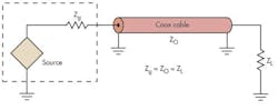
ZO = √(L/C)To achieve maximum power transfer over a transmission line, the line impedance must also match the source and load impedances (Fig. 6). If the impedances aren’t matched, maximum power will not be delivered. In addition, standing waves will develop along the line. This means the load doesn’t absorb all of the power sent down the line.
Consequently, some of that power is reflected back toward the source and is effectively lost. The reflected power could even damage the source. Standing waves are the distributed patterns of voltage and current along the line. Voltage and current are constant for a matched line, but vary considerably if impedances do not match.
The amount of power lost due to reflection is a function of the reflection coefficient (Γ) and the standing wave ratio (SWR). These are determined by the amount of mismatch between the source and load impedances.
The SWR is a function of the load (ZL) and line (ZO) impedances:
SWR = ZL/ZO (for ZL > ZO)

SWR = ZO/ZL (for ZO > ZL)
For a perfect match, SWR = 1. Assume ZL = 75 Ω and ZO = 50 Ω:
SWR = ZL/ZO = 75/50 = 1.5The reflection coefficient is another measure of the proper match:
Γ = (ZL – ZO)/(ZL + ZO)For a perfect match, Γ will be 0. You can also compute Γ from the SWR value:
Γ = (SWR – 1)/(SWR + 1)Calculating the above example:
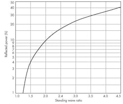
Γ = (SWR – 1)/(SWR + 1) = (1.5 – 1)/(1.5 + 1) = 0.5/2.5 = 0.2Looking at amount of power reflected for given values of SWR (Fig. 7), it should be noted that an SWR of 2 or less is adequate for many applications. An SWR of 2 means that reflected power is 10%. Therefore, 90% of the power will reach the load.
Keep in mind that all transmission lines like coax cable do introduce a loss of decibels per foot. That loss must be factored into any calculation of power reaching the load. Coax datasheets provide those values for various frequencies.
Another important point to remember is that if the line impedance and load are matched, line length doesn’t matter. However, if the line impedance and load don’t match, the generator will see a complex impedance that’s a function of the line length.
Reflected power is commonly expressed as return loss (RL). It’s calculated with the expression:
RL (in dB) = 10log (PIN/PREF)PIN represents the input power to the line and PREF is the reflected power. The greater the dB value, the smaller the reflected power and the greater the amount of power delivered to the load.
Impedance Matching
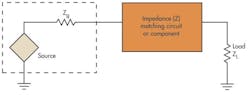
The common problem of mismatched load and source impedances can be corrected by connecting an impedance-matching device between source and load (Fig. 8). The impedance (Z) matching device may be a component, circuit, or piece of equipment.
A wide range of solutions is possible in this scenario. Two of the simplest involve the transformer and the λ/4 matching section. A transformer makes one impedance look like another by using the turns ratio (Fig. 9):
N = Ns/Np = turns ratioN is the turns ratio, Ns is the number of turns on the transformer’s secondary winding, and Np is the number of turns on the transformer’s primary winding. N is often written as the turns ratio Ns:Ns.
The relationship to the impedances can be calculated as:
Zs/Zp = (Ns/Np)2or:
Ns/Np = √(Zs/Zp)Zp represents the primary impedance, which is the output impedance of the driving source (Zg). Zs represents the secondary, or load, impedance (ZL).
For example, a driving source’s 300-Ω output impedance is transformed into 75 Ω by a transformer to match the 75-Ω load with a turns ratio of 2:1:
Ns/Np = √(Zs/Zp) = √(300/75) = √4 = 2The highly efficient transformer essentially features a wide bandwidth. With modern ferrite cores, this method is useful up to about several hundred megahertz.
An autotransformer with only a single winding and a tap can also be used for impedance matching. Depending on the connections, impedances can be either stepped down (Fig. 10a) or up (Fig. 10b).
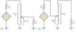
The same formulas used for standard transformers apply. The transformer winding is in an inductor and may even be part of a resonant circuit with a capacitor.
A transmission-line impedance-matching solution uses a λ/4 section of transmission line (called a Q-section) of a specific impedance to match a load to source (Fig. 11):
ZQ = √(ZOZL)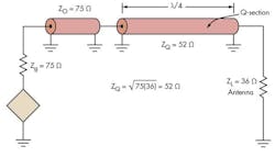
where ZQ = the characteristic impedance of the Q-section line; ZO = the characteristic impedance of the input transmission line from the driving source; and ZL = the load impedance.
Here, the 36-Ω impedance of a λ/4 vertical ground-plane antenna is matched to a 75-Ω transmitter output impedance with a 52-Ω coax cable. It’s calculated as:
ZQ = √(75)(36) = √2700 = 52 ΩAssuming an operating frequency of 50 MHz, one wavelength is:
λ = 300/fMHz = 300/50 = 6 meters or about 20 feet

λ/4 = 20/4 = 5 feet
Assuming the use of 52-Ω RG-8/U coax transmission line with a velocity factor of 0.66:
λ/4 = 5 feet (0.66) = 3.3 feetSeveral important limitations should be considered when using this approach. First, a cable must be available with the desired characteristic impedance. This isn’t always the case, though, because most cable comes in just a few basic impedances (50, 75, 93,125 Ω). Second, the cable length must factor in the operating frequency to compute wavelength and velocity factor.
In particular, these limitations affect this technique when used at lower frequencies. However, the technique can be more easily applied at UHF and microwave frequencies when using microstrip or stripline on a printed-circuit board (PCB). In this case, almost any desired characteristic impedance may be employed.
The next part of this series will explore more popular impedance-matching techniques.
Read more of this article that is part of the Analog Series: Back to Basics: Impedance Matching
About the Author

Lou Frenzel
Technical Contributing Editor
Lou Frenzel is a Contributing Technology Editor for Electronic Design Magazine where he writes articles and the blog Communique and other online material on the wireless, networking, and communications sectors. Lou interviews executives and engineers, attends conferences, and researches multiple areas. Lou has been writing in some capacity for ED since 2000.
Lou has 25+ years experience in the electronics industry as an engineer and manager. He has held VP level positions with Heathkit, McGraw Hill, and has 9 years of college teaching experience. Lou holds a bachelor’s degree from the University of Houston and a master’s degree from the University of Maryland. He is author of 28 books on computer and electronic subjects and lives in Bulverde, TX with his wife Joan. His website is www.loufrenzel.com.
Comment About the Article
To join the conversation, and become an exclusive member of Electronic Design, create an account today!

Leaders relevant to this article: