Reduce Inband Noise with the AVT Algorithm
In general data-collection/logging systems, some kind of sensor is attached to filter. Also, the signal-conditioning amplifier is used for signal modifications for gain/offset modification, followed by an analog-to-digital converter (ADC) and some kind of computer processing the data (Fig. 1).

In many of today’s applications, software performs most of the filtering and signal processing, with software-defined radio representing the extreme manifestation of signal-processing algorithms. Filtering is typically designed around a fast-Fourier-transform (FFT) algorithm, which can be susceptible to noise.
This file type includes high resolution graphics and schematics when applicable.
Ideally, the noise would have some stable frequency and amplitude, and be positioned outside the bandwidth of the actual signal that interests us. Then a bandpass filter, designed using an FFT algorithm, would filter out unwanted noise, and thus a clean signal could be handed over to the next stage for processing.
In reality, though, all system components will introduce errors, and the environment will introduce random and periodic noise that wreaks havoc on our system. The worst part is that some of the noise will end up in the useful data bandwidth, and it can’t be removed by any bandpass filter. Let’s analyze a simple system that does collect the data from a single sensor, like that shown in Figure 1.
For simplicity, let’s assume we’re measuring some voltage generated by the sensor. There’s no filter, the gain of the amplifier is set to 1, and offset is set to 0. Basically, we’re talking about a system in which the sensor is hooked up directly to the ADC, and we are trying to make sense of data.
In ideal world, the ADC produces a constant value that represents the sensor voltage. However, in a real-world scenario, environmental noise is picked up by sensor wiring and the sensor itself, in addition to thermal noise, ADC errors, and noise generated by the digital circuitry, power supply and voltage reference. Most of this noise is random in nature and doesn’t have any defined frequency or rise time. Also, some of the noise occurs at frequencies in the ADC’s bandwidth, characterized as inband noise. This fact eliminates all hope of using some kind of bandpass filtering to differentiate the noise from valuable signal. Hence, sophisticated FFT algorithms implementing filters won’t help.
At this point, some diehard FFT fans will protest that maybe they can play with coefficiency parameters and design some kind of useful filter. Please don’t do it; bandpass filters are useless in situations where inband noise is present. Yet there are techniques to improve the signal quality—we’ll compare them here using results obtained from running some random-noise-riddled data. The assumption is that this noise is inband and can’t be filtered; therefore, we’ll try to filter noise without using bandpass filters. First, let’s briefly describe the ways that can be achieved.
Filtering Noise by Data Averaging
This technique is based on collecting N samples and averaging those together to produce a single value that represents the actual voltage present at the sensor. As simple as it sounds, this technique works really well when FFT-based filters fail to give any improvements of data quality.
It is based on assumption of Gaussian noise distribution, where most random noise can be categorized. The larger number of samples N we use with this technique, the better the final signal approximation. Of course, we need to have some sane value of N to keep averaging circuits/software complexity down and practical. Therefore, we usually see N in the range of less than 100.
An interesting variation of this technique is when N is selected to be the power of 2. Basic shift registers/operations can be used, which greatly simplify the design, to implement divide-by-2 operations. Typical FPGA-based averaging implementation would be similar to Figure 2.
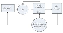
Here we have one m bit adder and n bit register, along with an imaginary shift register that’s implemented by just using the accumulator’s most significant n bits. The data-averaging state machine clears the accumulator before each cycle, manages the accumulation of N samples, and stores the result in an output register. The number of bits m used for the adder/accumulator is directly proportional to the number of samples:
m = log(N)/log(2) + n
This simple algorithm has a tiny footprint in the FPGA, especially when compared with a full FFT filtering implementation. For example, when N = 64 and n = 10, we just need a 16-bit adder and an accumulator to implement this algorithm with a small amount of additional logic.
Thanks to the simplicity of this algorithm, it can even be utilized in tiny microcontrollers lacking hardware-based division support. Several application notes that describe this implementation usually refer to this algorithm as a method for improving ADC resolution1,2,3.
Using Median Value as Effective Data
This is counterintuitive, but still an effective way of filtering data. It’s based on collecting N samples of data, sorting them, and selecting the value in the middle (the median). This technique is based on an assumption of noise being classified to have Gaussian distribution. Assuming a stable signal and Gaussian noise distribution of equally distributed opposite polarities, we will end up with a unique array of numbers—its median will correspond to a noise level of 0, assuming there are a large number of samples. While it’s easy to implement in software, the FPGA implementation could have a larger footprint than the averaging technique. Interestingly enough, this method of filtering isn’t used very much for data filtering, but produces better results than averaging as discussed below.
Statistical Filtering or AVT (Antonyan Vardan Transform)
This data-filtering algorithm isn’t described in literature to my knowledge; I came up with it while attempting to calibrate a precision system in a noisy environment. The necessity for this algorithm was apparent after I noticed that consecutive calibration attempts, using other data-filtering algorithms, produced different results each time. During the calibration process, all environmental factors in my setup were constant, exempt from noise. The algorithm is simple and can be implemented using the following steps:
1. Collect N samples of data.
2. Calculate the average and standard deviation of the dataset.
3. Drop any data that has a greater/smaller than average plus/minus standard deviation
4. Calculate the average on the remaining subset of data and present it as an output.
The advantage of this algorithm is that it doesn’t rely entirely on Gaussian distribution of noise.
It can easily detect and filter out infrequent random noise. This algorithm gets rid of obvious outliers or data points that have greater than one standard deviation change. By doing this, good data is filtered for the next stage or output. As a result, it improves data quality data quality presented for end use, and it doesn’t depend on Gaussian distribution of the raw data.
Most noise can be classified as having Gaussian distribution only when considering a large number of samples. In real life, we’re limited by time constraints, so we typically must generate meaningful data using relatively small sample sizes.
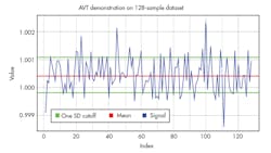
The basic AVT operation is demonstrated using sample data presented in Figure 3. It represents 128 samples of random-noise-riddled data; green lines mark normal data boundaries, and any signal outside this band is dropped to improve data quality. We declare all signal values outside this band as outliers and thus drop those values from all calculations.
Quantization of Methods/Algorithms
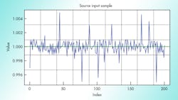
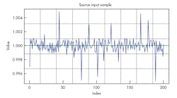
At this point, we need to do some kind of data analysis to compare the effectiveness of the three algorithms discussed in the article. To be impartial, we start with an original sensor reading being 1 and add to it random data in the form of noise at 0.001 maximum amplitude (0.1%). On top of it, we add some random noise at the 1% level (0.01 amplitude), but orders of magnitude less frequently. We generate this data using R script and save 100K samples (please see dataset.csv) and use this data in subsequent calculations. Figure 4 shows the first 200 samples from this dataset graphically. I would like to thank creators of R statistical computing software, who provided tremendous help in proving results and creating graphs in this article. You can download it for free.4 In addition, there’s a nice integrated development environment called R studio.5
We will analyze the results of filtering this data using those three methods/algorithms, utilizing N=32, 64, 128 samples and collecting results for 100 datasets. This functionality is provided by R script. This script produces a “var_result_dataset.csv” data file that describes the results of analysis. We are only interested in the error produced from those algorithms at various N values to quantifiably compare them (Fig. 5). In this graph, we indicate maximum, minimum, and standard deviation of the error in parts per million (PPM).
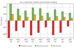
From this graph, we see that the AVT algorithm provides the best results in any sample rate compared with median and averaging algorithms. Please note that those analyses were done using pseudo-random noise generated by a script, which stresses the algorithms to generate subjective data for comparison. The results of implementaing those algorithms with real-life data are much more spectacular.
This file type includes high resolution graphics and schematics when applicable.
Vardan Antonyan is a senior hardware engineer at Aitech Defense Systems Inc., Chatsworth, Calif., with over 15 years of experience. He holds a patent and has published several articles.
References:
About the Author
Vardan Antonyan
Senior Hardware Engineer
Vardan Antonyan is a senior hardware engineer at Aitech Defense Systems Inc. (www.rugged.com), Chatsworth, Calif., with over 15 years of experience. He also has a patent. He can be reached at [email protected].
Comment About the Article
To join the conversation, and become an exclusive member of Electronic Design, create an account today!

Leaders relevant to this article: