An important design objective for voltage and current probes and current monitors is to determine a signal’s characteristics without significantly affecting the signal itself. In other words, the device should not load the signal source. In addition, a probe should not influence measurement accuracy, which implies low noise, wide bandwidth, and linear operation.
Voltage Probes
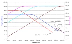
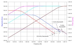
The accuracy of measurements made with almost any type of voltage probe depends on the ratio of the probe impedance to the signal source impedance. A conventional 10-MΩ 10:1 scope probe often is a good solution, although as shown in Figure 1, the typical 17-pF capacitance (impedance magnitude orange curve and phase shift pink curve) begins to increase the probe loading at frequencies higher than several kHz. For a source with low output impedance at high frequencies, such a probe can be useful up to a few hundred MHz.
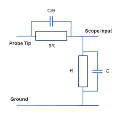
10:1 probes use a compensated attenuator design shown in Figure 2, which maintains the nominal ratio over a wide frequency range. So, even though capacitive signal loading increases with frequency, the amplitude and phase responses at the scope input remain constant, facilitating good pulse fidelity.
The impedance of 9R and C/9 in parallel is 9R/(1 + jωC), and the impedance of R and C in parallel is R/(1 + jω). As a voltage divider,
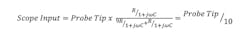
Ideally, there is no change in output for any frequency. In reality, this doesn’t happen because of stray capacitance, parasitics, and variations in the resistor and capacitor ratios. For example, resistors and capacitors have small sensitivities to voltage and temperature. Also, the scope input capacitance C is the composite of several smaller capacitances that have different sensitivities than the probe compensation capacitance C/9.
1:1 probes also are relatively common but have much lower bandwidth. Because of the 1:1 ratio, small signals are more easily measured but a compensated attenuator cannot be used. Instead, the input capacitance is the sum of the cable capacitance and the scope’s input capacitance—for example, the Tektronix P6101B 1:1 2-m probe has a 15-MHz bandwidth and 100-pF input C.
So-called transmission-line probes also are passive but can be used at multi-GHz frequencies. A scope’s 50-Ω input or a suitable 50-Ω thru termination used with a 1-MΩ scope input provides a matched load for a 50-Ω cable. This means that looking into the open end of the cable, the impedance is very nearly a pure resistance—the capacitance is very small. By adding a series resistor at the input, a low-capacitance attenuator is formed.
Figure 1 shows the input impedance magnitude (purple curve) and phase shift (brown curve) for a 10:1 transmission-line probe with 0.25-pF input capacitance. Although this type of probe is low cost and accommodates very high frequencies, its resistive loading can be too high for some supplications.
Many scope companies have developed active probes that reduce loading at high frequencies. Typically, this is accomplished in two ways. These probes have very low input C and many of them also feature input resistance in the 50-kΩ to 1-MΩ range. The combination minimizes loading at GHz frequencies. Figure 1 shows the magnitude (blue curve) and phase shift (aqua curve) corresponding to the input impedance of a 1-MΩ//0.9-pF active probe.
For a more detailed discussion of passive and active voltage probes, refer to Reference 1.
Current probes
Hinge-opening or slide-opening current probes are convenient to use because the current-carrying circuit doesn’t have to be broken—just clip the probe to the wire and measure the current. Often this type of probe is used with a multimeter. Scope manufacturers also make these probes, some specified from DC to 100 MHz.
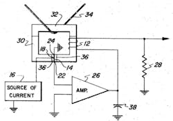
U.S. patent 3,525,041 (1970) Magnetic Field Measuring Method and Device Effective Over A Wide Frequency Range describes a current probe similar to the (discontinued) Tektronix A6302, which used a small split-core transformer for AC current up to 50 MHz and a Hall-effect sensor for DC and low-frequency current to 20 A. As shown in Figure 3 (Figure 2 in the patent), the probe uses both transformer coupling 12 and a Hall-effect device 14.
Courtesy of Patent 3,525,041
The small transformer core 30 and 32 is split so that it can be placed around the current-carrying wire. As Figure 3 shows, Hall device 14 is subject to the total magnetic flux because the device is mounted in a gap in the core. Elements 36 are thin, high-resistance ferrite layers added to avoid shorting out the Hall device. However, it is the current feedback from amplifier 26 that is most interesting.
By way of background, before high-impedance electronic circuitry was common in instruments, potentiometric techniques were used to achieve high-accuracy DC voltage measurements. The basic idea is to use a null detector to indicate the difference between the unknown voltage and a separate voltage source. When the unknown voltage and the separate source have equal values, zero current will flow into the detector—the voltages are exactly balanced, so even a relatively low input impedance detector doesn’t load the unknown source.
In addition to achieving the equivalent of high input impedance, the technique has a more subtle benefit. Balancing the unknown voltage means that the null detector always operates at the same point. Even if the detector is nonlinear, because the same (zero) current point indicates balance, the measurement remains accurate.
This technique has been applied to the magnetic circuit in Patent 3,525,041. The output from the Hall device drives amplifier 26, which is band-limited by capacitor 38. The amplifier output current is applied to winding 12 and develops a voltage across shunt resistor 28. The flux developed by the coil counteracts the flux associated with the unknown current flowing in wire 34—the current being measured. This means that the Hall device always operates near zero flux, so the device’s inherent nonlinearities and those of the amplifier 26 and the core 32 are not important.
Also, because the feedback from amplifier 26 extends from DC to some low frequency, the core 32 will not be biased. This is critical because to achieve very high-frequency operation, a small, easily saturated core must be used. Bucking out the low-frequency field from the current in wire 34 allows high-frequency signal components to couple to the transformer winding 12 and be superimposed on the signal across shunt resistor 28. And, as in normal transformer operation, the secondary high-frequency current flowing in winding 12 produces magnetic flux that cancels the flux caused by the primary high frequency current flowing in conductor 34.
Many improvements have occurred over the years. For example, patent 5,477,135 (1995) Current Probe references patent 3,525,041 but adds circuitry to make the probe self-calibrating and capable of compensating for Hall-effect device temperature sensitivity. Nevertheless, probes that combine transformer coupling and a Hall-effect device are similar to the design described in the 1970 patent.
Current monitor
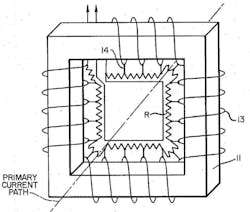
A different kind of measurement problem is addressed by Pearson current monitors. As occurred for current probes, the theory and original development were done decades ago. In this case, patent 3,146,417 (1964) Transformer describes work by Dr. Paul A. Pearson to extend and linearize a current transformer’s frequency response. The patent includes several detailed drawings and a thorough description of theory as well as a preferred implementation. Figure 4 (patent Figure 1) gives a good overview of the basic idea.
Courtesy of Patent 3,146,417
The original Pearson current monitors did not use a split core so it is necessary to break the current-carrying circuit to pass the wire through the open center of the monitor. In addition to measuring current in a wire, these monitors can be used to measure the current in an electron beam passing through the aperture. Today, Pearson-type monitors are made in two styles: one with a split core and one with a solid core.
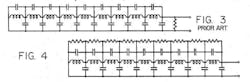
As discussed in the patent, the winding 13 is inductive and has capacitance from each turn to the core (11) as well as from each turn to other turns. Figure 5 (patent figures 3 and 4) compares the equivalent circuit of prior art (Figure 3) current transformers and the circuit representing the Pearson approach (Figure 4).
Courtesy of Patent 3,146,417
A prior-art transformer presents many opportunities for the stray and parasitic capacitances to govern its frequency response. Termination is at the output and can only be an approximate match. In contrast, the Pearson transformer consists of multiple smaller terminated transformers in series. Figure 3 shows the multiple connections to a tapped resistance that causes each section to have a broad, damped frequency response.
The bandwidth is further extended by constructing the transformer as a tapped resistive transmission line in parallel with the tapped winding. In some models, a series resistor is added to the distributed transformer load to achieve 50-Ω overall impedance. Bandwidths to 300 MHz and current levels of 500 kA are available in different models.
Summary
Although they are a critical part of a test setup, probes often don’t receive a lot of attention. And, many times, it’s not warranted anyway. Relatively low-speed and low-impedance signals don’t demand much care. In general, if a 10:1 probe is adjusted to have a good pulse response, the readings it gives will be accurate.
That’s not the case for signals with high source impedance or high-speed edges or for signals that are exceptionally large—10s of kA or kV. For very large signals, operator safety is the first consideration—next comes instrument safety, and eventually, measurement accuracy. High source impedance and/or very high frequencies probably require an active probe. A high-speed signal with low source impedance may allow use of a transmission-line probe.
Precise high bandwidth high-current measurements are the domain of the Pearson current monitor. For example, the Model 6600 handles up to 2,000 A and frequencies from 40 Hz to 120 MHz. It supports 5-ns 10-90% rise/fall times, has a 50-Ω output impedance, and measures 4.38 inches in diameter with a 2-inch diameter aperture. The output sensitivity is 50 mV/A ±1% into 50 Ω.
Reference
- Lecklider, T., “Scope Probes with Attitude,” EE-Evaluation Engineering, November 2009.
About the Author

Tom Lecklider
Comment About the Article
To join the conversation, and become an exclusive member of Electronic Design, create an account today!

Leaders relevant to this article: