Part Two: Linear Superposition Speeds Thermal Modeling
Part one of this series, published in the January 2007 issue, discussed how to use linear superposition in the steady-state analysis of multiple heat-source systems. However, linear superposition also can be used in the time domain, which is very useful. This means if you have a thermally linear system, you don't have to be limited to steady-state temperature predictions. The rules remain pretty much the same: The individual temperature responses in your system have to be proportional to individual heat-source values and, except for those heat sources, all the other boundary conditions have to stay fixed over the time and space of interest.
The Concept
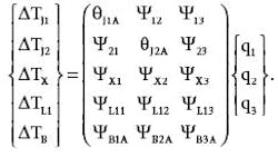
Consider the case of a multiple heat-source system that can be described in steady state by a matrix equation. In such a case, the thermal transient response of the system can be determined merely by turning each matrix element into its corresponding time-varying counterpart. For example, the matrix equation cited in part one described a power system model (refer to Fig. 1 in part one) with three heat sources (q1, q 2and q)3 and five points of interest on the pc board for which temperature calculations were desired (TJ1, TJ2, TX, TL1 and TB). These temperatures are calculated by the following matrix equation:
where the theta coefficients (θJ1A and θJ2A) represent “self-heating” terms, and the psi coefficients (ψ12, ψ13, etc.) represent “interaction” terms.
We can use this same power system model to illustrate how the matrix is modified to obtain the transient response of the system. But to make the calculations easier to follow, we'll simplify the power system model by assuming a two heat-source system and calculate just two temperatures on the pc board. Making those changes along with the switch to time-varying elements gives us this transient matrix:
where Δq1-STEP and Δq2-STEP represent step changes made to the two heat (or power) sources.
Now, each of the theta matrix elements is a complete thermal transient response curve. The main complication is that every time any heat source changes its value, then every other response must also make a simultaneous adjustment — a fair amount more work than if you're just tracking the temperature of a single device.
So the bookkeeping may get tedious, but the method is straightforward. We can calculate the values of the time-varying temperature vector of Eq. 2 using Excel. But to get to that point will require a whirlwind course reviewing several separate, but ultimately related, topics including Cauer networks, Foster ladder networks, Reciprocity Theorem and time-domain superposition.
Thermal Transient Networks
Fig. 1 illustrates a hypothetical two-input grounded-capacitor, sometimes known as Cauer, thermal network. Cauer networks are of interest because in the thermal world, they are the natural representation of the physics. Nodes store energy, represented by capacitors to ground, and heat flow between nodes is represented by resistors. Unfortunately, although these are easy to draw, and the individual resistor and capacitor values may be easy to calculate (at least if you thought about where the heat was flowing when you drew the network), they're a pain to analyze with inexpensive tools.
Consider instead the ladder network shown in Fig. 2. These networks, called Foster ladders, are easy to analyze and implement. In response to a sudden application of constant power (ΔqJ), the response of the end node is merely the sum of a bunch of exponentially decaying terms, as in:
where the Ri terms represent the resistors in the Foster networks, and the τ iterms represent the associated R-C constants. Using Excel array notation and the Insert:Name:Define menu feature, this can be expressed very elegantly. For example, defining:
the temperature rise at the time specified in cell A4 is computed in Excel by the array formula:
{=power*SUM(resistances*(1-EXP(-A4/taus)))}.
The saving grace of linear thermal networks such as Fig. 1, is that there is generally a mathematically equivalent Foster solution for every node in the system. Further, you probably only care about results at the heat-input locations, and maybe another location here or there. I do need to emphasize that when you find the corresponding Foster ladder that goes with the heat input at TJ1, whether it's from a Cauer model simulation or perhaps directly from an experimental curve, it will have a bunch of nodes or “rungs” as in Fig. 2 that don't mean anything physically; but, it will have one node, the end node, that behaves exactly like TJ1 over the entire time domain.
Transient-Response Curves
The transient-response curve mentioned previously simply refers to what you get if you're tracking the temperature at some point in your system, in response to a step of constant power applied to some (perhaps other) point in your system. Fig. 3 illustrates a set of transient-response curves for a two-source system.
Two of the curves are labeled “self-heating curves” and one is labeled “interact.” In a completely general way, there should be four curves (since there are four matrix elements for a 2-by-2 matrix). Although not mentioned in part one of the article series, when dealing with truly linear networks, the Reciprocity Theorem states (for our purposes) that the theta matrix, in theory, will be symmetric. That is, in our 2-by-2 matrix the two source-to-source interaction curves will be identical — true even when the self-heating curves themselves are not at all identical.
I've tested lots of real-life systems, and this theoretical reciprocity/symmetry is usually a good approximation for semiconductor devices. Obviously, if you have any doubts, try to get both curves on their own. But for this example, we will use a single interaction curve interchangeably between the two sources.
Characterizing the System
Part one of this article discussed how you could use either experiments or some sort of simulation of your steady-state self-heating and interaction responses to fill in the theta matrix. The same applies here. Thus, your first step is either to actually go down to the lab with your prototype application and do some live thermal transient measurements (an art in itself), or create a representative Cauer network model of your system and use it as a lab to run a set of experiments, which means you'll need a circuit simulator.
A third option is to use high-powered finite-element or computational fluid dynamics code to do a transient simulation of your system. However you go about it, the goal is to generate a set of thermal transient-response curves at each point of interest to unit-steps of constant power at each heat source. Reciprocity can save a lot of work, but when in doubt, measure your interaction curves both ways. Remember to normalize the curves so they are on a per-watt basis.
Once you have a complete set of transient-response curves, tabulate the data on a logarithmic time scale. In my lab and simulations, I typically pick a ratio, say 15√10, and then space my data points as close as I can to that ratio from 100 µs all the way out to 1000 sec. For the data in Fig. 3, that would give me 15 equally spaced points per decade times seven decades, which would equal 105 points total. (In my lab, I actually log data at a uniform 8-µs interval and then throw most of it away. In simulations, I can more easily solve for and save just the required points.)
Here is when Excel can really be put to use. To fit Foster network models to the data of Fig. 3, you probably don't need more than one time constant for each order of magnitude of time data available to you. (I've rarely seen data for which this doesn't provide a decent fit, though using more hardly costs any additional effort; unless you go overboard, Excel can easily handle more.)
With the curves in Fig. 3, that would mean choosing time constants at 0.0001 sec, 0.001 sec and all the way up to 100 sec. Fig. 4 shows how: list the time constants (taus) in a column (I3:I10) and, next to them, allow three more columns for the Foster resistances (J3:L10). Columns E through G are the computed fits, each column coming from its own specific version of Eq. 3. Cells E1, F1 and G1 are root-mean-squared errors (RMSE) for each column; E1, for instance, contains the formula:
{=SQRT(SUMSQ(E4:E100-B4:B100)/COUNT(E4:E100))}.
Now select Tools:Solver. For each curve in turn, point Set Target Cell: to its RMSE value, click Min, select the corresponding column of resistances for By Changing Cells: and hit Solve. Almost any starting guesses will do; the resistances shown in cells J3:L10 of Fig. 4 are the converged, least-squares best-fit values. You saw how well this worked in Fig. 3 if you noticed the curves superimposed on top of the raw data points: Those are the best fit results.
Single-Source Time Superposition
This next technique should just be a review of something you learned a long time ago — namely, how to apply time-domain superposition to the analysis of a time-varying heat source (or current source using the electrical analogy). If you understand how this works for a single heat source, it won't be such a stretch to see how it adapts to the multiple heat-source situation. Fig. 5 illustrates the basic stages:
-
Begin by “squaring up” your actual time-varying power input. The resolution of the squaring basically depends on how accurate you need to be at critical points. Basically, replace large regions of complicated stuff with a single rectangular power pulse that contains the same energy, anywhere you don't care about the temperature details within that region.
-
Convert those individual square power pulses into steps of increase or decrease as you move from one constant region to the next (including zero-power regions).
-
Each step-change of power turns into its own power-scaled version of the transient-response curve for the heat source. It starts when the change is applied and ends when the simulation ends.
-
Sum up these individual response curves algebraically (meaning that increases add and decreases subtract). Clearly, only pulses up through any particular moment of interest affect the cumulative temperature change; the farther along in time you go, the more steps you have to track.
Putting It All Together
In the final step in our analysis, we convert matrix Eq. 2 back into two separate equations that describe the temperatures at the two junctions of our 2-by-2 example:
where θJ1_SELF(t) and θJ2_SELF(t) represent the two curves in Fig. 3 labeled “q1 self avg” and “q2 self avg,” respectively, and ψ1-2(t) represents the “interact” curve.
Recall that these equations predict the temperature rise at the two locations of interest to us here, relative to some reference (in this case, it's going to be ambient). As I've already suggested, the idea is that any time either of the power sources change value, either by increasing or decreasing, you have to start adding in new step solutions on top of however many previous steps you've made — and this is crucial: Don't stop adding in the previous steps just because you've started a new step.
You can also see why you have to start a new time-step solution for every location, whenever any power source changes, because every location is affected by every power source. Eq. 6 is a mathematical statement of these ideas, as applied to Eq. 4, utilizing the concept of the unit-step function, and where the summation is taken over the entire set of times at which power changes at either source:
where u(x) = 0 for x < 0 and u(x) = 1 for x ≥ = 0.
The way I usually implement this in Excel is illustrated in Fig. 6, which includes liberal use of variable names to make the formulas as mnemonic as possible. The following tables, shown in Fig. 6, highlight major points:
Table 1 is simply the Foster model we derived earlier.
Table 2 is the input table of all the times at which either of the power sources change value, along with the power values. I've plotted those two power versus time functions on the chart in Fig. 6 on the secondary Y axis. Cells O7:Z8 immediately below Table 2 are the changes in power at each of those times, needed in subsequent formulas. (Note that there's no correlation between the waveforms in Fig. 6 and those in Fig. 5.)
Table 3 implements the unit-step function using an array-formula “if” statement (where time is the name of cell O11 and change_at is the name of the entire block O4:Z4):
{= if ( time > change_at, time - change_at, 0)}.
Table 4 uses the following two array formulas to compute the contribution of each individual time-step of Table 3 toward the total (compare these with Eqs. 4 and 5):
{=SUM((P7*q1_R_s+P8*interact_R_s)*(1-EXP(-P11/taus)))}
{=SUM((P7*interact_R_s+P8*q2_R_s)*(1-EXP(-P11/taus)))}.
The first of those two formulas actually appears in cell P13, and though it is an array formula, it returns just the single value seen in cell P13. The formula is then copied into every other cell of row 13 in Table 4, and similarly with the second formula and row 14. Conveniently, (1-EXP(-P11/taus)) contributes exactly zero for a zero argument, thus simplifying the use of the unit-step function, which stuffs a zero into every relative time value of Table 3 for times later than the time of interest).
Finally, Table 5 is the only true Excel “table,” via the formula: {=TABLE(,O11)}.
Table 5 calculates the final values of TJ1 and TJ2 at the selected times. To construct this table, you list in cells J14:J35 all the times for which you'd like results, and in cells K13 and L13, input the (nonarray) formulas:
=SUM(T1_terms)+ambient, and =SUM(T2_terms)+ambient.
Then select cells J13:L35, pick Data:Table from the menu, and for the Column Input Cell, pick O11. Note in the example that the yellow highlighted time entries happen to be some, but not all, of the exact times at which power levels changed in Table 2. I added some extra time values between some of the change_at points where I was interested in more detail. If you want results at more time points, simply lengthen Table 5.
Extending the Technique
Though this example was just a two-source problem, the technique can be extended to an arbitrary number of power sources. The main points to emphasize in adding more sources are these: You must have interaction curves for all pairs of source and location (so that the number of columns of Table 1 increases geometrically with the number of sources — though the principle of reciprocity may be able to reduce the number somewhat), and you need an entry in Table 2 each time any power source changes value. Finally, if you take advantage of Excel's naming capability, you can keep the formulas fairly mnemonic, and thus easy to maintain.
When reading part one of this article series, you may have scratched your head a bit and wondered why you'd even bother breaking down a sophisticated steady-state simulation into individual linear responses, when you could probably just as easily change your power inputs in the simulation and rerun it (especially if you've got a nonlinear simulation). Well, that was really just to set the stage for the thermal transient problem, because when you throw time into the mix, the possibilities are more than endless.
Not only can you change the power inputs at different locations, but you can turn them on and off in different sequences; they might be synchronized and periodic in one application, and totally random or asynchronous in another. A full-blown transient simulation, even in a completely linear system, can take hours to run. Having to rerun it every time a single power source changes amplitude or timing quickly becomes prohibitive.
Comment About the Article
To join the conversation, and become an exclusive member of Electronic Design, create an account today!

Leaders relevant to this article: