Choosing the Proper Parameters in Frequency Spread Spectrum (FSS) Design

This article is part of the TechXchange: Delving into EMI, EMC and Noise.

Members can download this article in PDF format.

What you’ll learn:

The key parameters of the FSS technique and their impact on EMI performance.
How to evaluate FSS performance using simulation, ICs, and a signal generator.

Frequency spread spectrum (FSS) is a technique that’s been widely used in power-conversion designs to reduce electromagnetic-interference (EMI) noise. But optimizing EMI without compromising on other aspects of the design can pose some challenges.

Many different parameters must be considered in the context of FSS design, including the modulation shape, frequency, and depth, all of which have varying impacts on the EMI spectrum. This guide runs through three different methods to evaluate FSS technologies and optimize these parameters.

The Fundamentals of Frequency Spread Spectrum

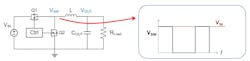
The active switches in a power converter operate at high frequencies, generating high transient-voltage (dV/dt) nodes and high transient-current (di/dt) loops in the circuit. These unavoidably lead to undesired EMI noise flowing into the circuit. EMI can wreak havoc in power electronics, harming performance and raising the risk of malfunctions and even a total system failure. Figure 1 shows the switching waveform of the dV/dt node in a buck converter.

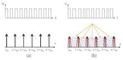
1. The active switches in a power converter generate high dV/dt nodes.

When the switching frequency (f_SW) is fixed, the EMI spikes can spike at the fundamental and harmonic frequencies of f_SW (Fig. 2a). Industry standards for EMI—e.g., CISPR 25—require the peak noise spectrum to not exceed a given threshold. The main principle of the FSS technique is to modulate the power converter’s f_SW to distribute the noise energy in the spectrum, which reduces the peak EMI noise spectrum (Fig. 2b).

2. The fundamental and harmonic components in the frequency spectrum (a) and FSS technique decrease the peak noise spectrum (b).

For a long time, it was unclear whether FSS technology was a winning strategy since it reduces the peak values of the EMI spectrum to meet industry standards rather than reducing the total noise energy. While it was not a sure-fire solution at first, FSS has become broadly adopted, and it can work within both the frequency domain and time domain:

In the frequency domain, the circuit plagued by EMI is sensitive to only a few frequency ranges, and the FSS technique reduces the power density on these ranges.
In the time domain, the circuit exposed to EMI has a settling time; interference is reduced if the time interval for the sensitivity frequency band signal is shorter than the settling time. The FSS technique decreases the time interval of the sensitive frequency band.

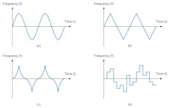
In recent years, various methods of frequency spread spectrum with different modulation shapes have been proposed, and they work by varying the frequency versus the time relationship. Figure 3 shows the typical FSS modulation waveforms, including sinusoidal, triangular, Hershey Kiss, and pseudo-random, each of which impact the performance of the FSS differently.

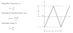
3. Various FSS methods have been proposed, such as sinusoidal (a), triangular (b), Hershey Kiss (c), and pseudo-random (d).

In addition, Figure 4 shows parameters such as modulation frequency (f_M), span, and the modulation index (m) that impact the performance of the FSS, where T_M is the modulation period. To optimize these characteristics, it’s necessary to carefully evaluate them through the lens of the specific FFS technology.

4. Typical parameters in the FSS technique include fM, span, and m.

Evaluating the Performance of Frequency Spread Spectrum

There are three main methods to evaluate FSS performance: simulation using software tools, evaluation via hardware, and using a signal generator. These methods are described in further detail below.

Method 1: Simulation

A straightforward approach to evaluating FFS is to generate the switching waveform using a circuit simulation tool and then analyze its spectrum. However, the simulation tool typically only provides the fast Fourier transform (FFT) result, which is different from the spectrum measured by an EMI receiver in practice. Therefore, FSS simulation should be based on the principle of EMI receivers instead of FFT.

Figure 5 shows the diagram of a stepped-frequency EMI receiver, where the key blocks include the mixer, the intermediate-frequency (IF) filter, envelope detector, and EMI noise detectors.

5. The key blocks of a stepped-frequency EMI receiver include the mixer, IF filter, envelope detector, and EMI noise detectors.

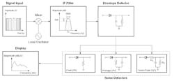
The EMI receiver can convert the input signal via a mixer and local oscillator (LO) to the IF. Since the LO frequency is tunable, the entire input frequency range can be converted to a constant IF by varying the LO frequency. An IF filter is applied to extract the components around the targeted frequency.

The resolution of the analyzer is then determined by the IF filter. EMI standards (e.g., CISPR 16) regulate the IF filter’s transfer gain requirement. In the simulation, the IF filter can be modeled as a bandpass Gaussian filter, where the transfer gain can be calculated with this equation:

The RBW coefficient, represented by c, can be calculated with the following equation, where RBW is the EMI receiver’s resolution bandwidth:

The IF filter’s output is first fed to an envelope detector; then the detector extracts the magnitude of the input signal overtime (Fig. 5, again). This detector can also be modeled in the simulation with a transfer function.

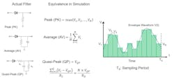
The noise detector is the last stage of the EMI receiver. Figure 6 shows the EMI receiver that can display the peak value, average value, or quasi-peak (QP) value regulated by various EMI standards. These standards are achieved with different analog filters, and the behaviors can be modeled in the simulation.

6. Noise detectors and their equivalences can be modeled in simulation.

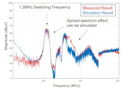
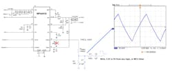
Using the stepped-frequency EMI receiver, it’s possible to emulate the EMI receiver with a simulation tool. Figure 7 shows a comparison between the measured EMI spectrum and the simulated spectrum based on the MPQ7200-AEC1, a buck-boost LED driver. The simulation results show that the spread-spectrum effect corresponds with the measured results.

7. The simulated EMI corresponds with the measured EMI.

Obtaining simulated results is typically a time-consuming task. Thus, predicting the impact of different FSS parameters may require a more convenient evaluation method using ICs.

Method 2: Hardware Evaluation

For many IC devices, the frequency-spread-spectrum parameters are configurable via a digital interface. Therefore, using an evaluation board with a digital interface simplifies the process of checking the EMI performance of different settings.

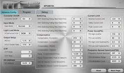
Figure 8 shows an example with the configuration table of the MPQ8875A-AEC1, an integrated buck-boost converter with a digital interface that supports parameter configuration. FSS can be enabled or disabled, and its f_M and span can be adjusted as well, enabling the performance to be evaluated digitally.

8. The MPQ8875A-AEC1’s configuration table supports parameter configuration.

For products lacking a digital interface, an analog pin can be used to set f_SW. An external circuit can be designed to make f_SW follow a triangular waveform, where f_M and span are determined by the R and C values. Figure 9 shows the external circuit of the MPQ4430, a step-down switching regulator, to configure f_SW.

9. The external circuit of the MPQ4430 can be used to configure the switching frequency.

Method 3: Signal Generators

There are times when it’s possible to configure the frequency spread spectrum setting via a digital interface or analog pin, or it’s necessary to evaluate parameters that aren’t included in the IC setting. In these cases, a signal generator can be utilized to perform the evaluation.

The signal generator’s output is connected to an EMI receiver for analysis. With the proper settings, the signal generator can also generate switching waveforms using various FSS techniques. In this way, the noise source’s EMI spectrum is emulated and can be directly displayed with a PC connected to the EMI receiver. The result without FSS could be set as a baseline to compare the noise-reduction effort of various FSS techniques.

Most signal generators support frequency modulation (FM) to emulate the sinusoidal or triangular frequency spread spectrum. For pseudo-random or other complex modulations, the waveform file may be generated with the associated waveform editor. The amplitude of the signal should be small enough; it’s recommended to be about 100 mV to protect the EMI receiver’s radio-frequency (RF) input.

Dialing in Frequency Spread Spectrum to Reduce EMI

Frequency spread spectrum is one of more popular ways to reduce EMI in a power system. However, care must be taken when choosing the modulation frequency, the frequency span, and the shape of the waveform. Otherwise, performance can be left on the table.

Modulation Shapes

Important to keep in mind is the modulation shape. Figure 10 shows the spectrum of different frequency spread spectrum modulation shapes. For example, the spectrum of sinusoidal modulation has a spike at the edges, while the Hershey Kiss modulation provides a much flatter spectrum.

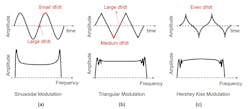
Consider the slew rate of the frequency (df/dt) for sinusoidal modulation, where df/dt is small at the sides of the entire frequency range, and df/dt is large at the center frequency. This indicates that f_SW isn’t spread out well at the edges, resulting in a spike at the edges. For triangular modulation, although df/dt at the center frequency exceeds df/dt at the edge frequency, df/dt is more constant compared to sinusoidal modulation, resulting in a flatter spectrum.

To reduce peak EMI noise, a flat spectrum is recommended, and df/dt and time should be constant. The performance of triangular modulation is typically sufficient and easy to implement, leading it to be widely applied in power-supply design.

Modulation Span, Frequency, Index, and RBW

Other features, ranging from the modulation span, frequency, and index to the RBW, can also impact EMI performance to varying degrees. Figure 11 shows the EMI spectrum with different modulation spans varying between 1% and 40%. The red line is the envelope of the noise spectrum where FSS is disabled, and it serves as the baseline.

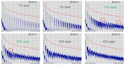
11. The EMI spectrum for various modulation spans ranges between 1% and 40%.

While a larger span achieves better EMI performance, a span exceeding 20% tends to not yield significant improvement. In fact, a large FSS span can impact the stability of the converter and overlap with sensitive bands like the AM band (530 kHz to 2 MHz). Therefore, a 10% to 20% span is typically selected.

Increasing the frequency span also helps reduce the EMI noise until the adjacent harmonics start to overlap, which occurs at a frequency close to f_SW/span, indicated by the red circle in Figure 11.

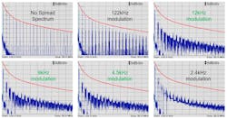
Selecting the modulation frequency also plays into EMI performance. Figure 12 shows the EMI spectrum for various modulation frequencies. For a fixed RBW, the optimal modulation frequency for peak EMI noise is typically around RBW in practice. In this case, RBW is selected at 9 kHz. The optimal modulation frequency is also about 9 kHz. If RBW and the span (or ∆f) is fixed, an optimal m is achieved.

12. The EMI spectrum for various modulation frequencies depends on RBW and span.

To analyze the noise-reduction effect of varying m, consider two cases with a very large m (Fig. 13a) and a very small m (Fig. 13b).

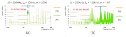
13. Shown is the EMI spectrum of a 2-MHz square waveform with a very large m (a) and a very small m (b).

The results are based on the EMI spectrum of a 2-MHz square waveform with different frequency spread spectrum modulations, output by a signal generator and analyzed by an EMI receiver. If m is very large, it means the f_SW is almost constant during the interval when the EMI receiver captures the data related to RBW. As a result, the frequency is not spread at all. On the other hand, if m is too small, there are only a few steps of f_SW. The energy is concentrated on these steps and cannot be evenly distributed across the span.

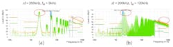
For different RBW settings, the optimal m is different. Based on CISPR regulation, for band B (150 kHz to 30 MHz), RBW is equal to 9 kHz; for band C and D (30 MHz to 1 GHz), RBW is equal to 120 kHz. There’s a tradeoff for f_M selection: At f_M = 9 kHz, the EMI performance of the low-frequency band is optimized, while at f_M = 120 kHz, the high-frequency band’s EMI is optimized (Fig. 14).

14. This is the EMI spectrum of a 2-MHz square waveform with fM = 9 kHz (a) and fM = 120 kHz (b).

EMI Detectors

To pass EMI tests, both the peak and average EMI noise must meet regulations. Similar to peak noise, the impact of the FSS parameters on average EMI noise can also be examined using a signal generator and EMI receiver. Table 1 shows a comparison of the results of noise-reduction performance with various FSS parameters and noise detectors.

Table 1: Noise-reduction performance with various FSS parameters and noise detectors.

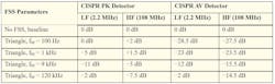
Unlike with peak noise, the attenuation of average EMI noise is better with a larger m due to the significantly higher data-acquisition interval for the average detector compared to the peak detector. Even with a large m, the energy remains evenly spread across the FSS span. When selecting the FSS parameters, it’s more critical to select a proper f_M based on its impact on peak EMI noise.

Dual-Modulation FSS

As previously established, if the modulation frequency is close to RBW, optimal FSS performance is achieved in the frequency band where RBW is applied. Figure 15a shows a modulation waveform with dual frequency components that’s proposed to reach a balance between high- and low-frequency performance. Figure 15b shows that the waveforms with different high-/low-frequency component ratios can be imported into a signal generator to be further processed by the EMI receiver.

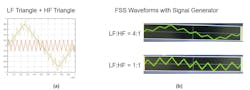
Table 2 reveals the performance of dual-modulation frequency spread spectrum.

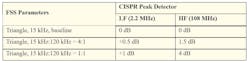
Table 2: The performance of dual-modulation FSS.

Compared to FSS with single-modulation frequency, the dual-modulation technique helps improve the high-frequency band EMI performance, while the low-frequency EMI becomes degraded.

As power converters with increasingly higher switching frequencies are developed today, the high-frequency EMI poses notable challenges. Dual-modulation FSS, which improves the high-frequency EMI noise attenuation, has been applied in several power ICs from MPS, such as the MPQ4371-AEC1.

Keep it Down: Easing EMI in Noisy Environments

Frequency spread spectrum is an effective method for EMI noise reduction. But noise-sensitive applications, such as radar sensors and Class-D audio amplifiers, have their own sensitive frequency bands. The FSS technique must not induce extra noise on these bands.

The RF rails of a radar sensor are sensitive to power-supply ripple and noise in the baseband (10 kHz to several MHz) because these supplies feed the phase-locked-loop (PLL) circuit, baseband analog-to-digital converter (ADC), synthesizers, and various other blocks (Fig. 16). So, in these cases, FSS parameters require special consideration to prevent degrading normal operation.

16. The FSS technique must prevent extra noise in the baseband of radar sensors.

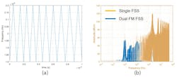
Figure 17a shows a waveform for dual FM frequency spread spectrum, which is one approach to reducing the impact of baseband noise performance by modulating f_M. The frequency spectrum of dual FM FSS is compared with a single FSS in Figure 17b, where the frequency spectrum of a square waveform is modulated with a fixed f_M. A significant component occurs at f_M and its harmonics, which can influence the baseband noise performance. The peak value around f_M is greatly reduced and benefits the radar sensor’s noise performance.

17. The dual FM FSS modulation waveform for the spectrum of single FSS (a) and dual FM FSS (b).

Since the audio band for Class-D amplifier applications (20 Hz to 20 kHz for the normal audio range, or 20 Hz to 40 kHz for the high-resolution audio range) are sensitive to power-supply noise, the FSS technique doesn’t influence noise. This band isn’t very wide, and a straightforward method to reduce the impact of baseband noise performance is to set f_M beyond the audio band. Typically, f_M can be implemented between 35 and 50 kHz for the 20-kHz band, or between 70 and 100 kHz for the 40-kHz band.

Read more articles in the TechXchange: Delving into EMI, EMC and Noise.