Using SPICE to Measure Effective Capacitor Ripple Current

Robustness in a power-supply design is based on predictable, long-term service life. In conventional switch-mode power supplies (SMPS), this is most often dictated by the characteristics of aluminum electrolytic capacitors. However, these components, sometimes called Al-Ecaps, degrade over time. As a result, accurate estimation of capacitor lifetime requires precise calculation of the ripple current, which is the primary cause of that degradation.

One approach is to use oscilloscope-captured data from a power supply and Fast Fourier transform (FFT) analysis in LTspice to evaluate all factors that can cause current ripple. With this approach, verifying the effective ripple current and resulting internal temperature rise of the capacitor can be achieved without resorting to expensive equipment or relying on oversimplified approximations. This article provides power-supply designers with a step-by-step guide.

Estimating the Lifespan of a Power Capacitor

Unlike other components, aluminum electrolytic capacitors use a liquid electrolyte that’s subject to diffusion and evaporation, making it the primary life-limiting component and determining factor for a system’s reliability and longevity. For these capacitors, the estimated lifetime (LX) is modeled as a product of the rated life specified by the manufacturer and a set of acceleration factors that account for electrical and thermal properties specific to the application.

The general formula for figuring this out is expressed as:

The rated life of the capacitor or its designated lifespan is represented by L₀, while K_T is the thermal acceleration factor, K_V is the voltage acceleration factor, and K_R is the ripple current acceleration factor. As a result, Equation 1 can vary depending on the capacitor manufacturer. One example is shown in Equation 2:

While L_X and L_O are in terms of hours, K_T is the ambient temperature acceleration factor, T_O is the upper limit of the category temperature range in degrees Celsius, T_X is the actual ambient temperature in degrees Celsius, and ΔT_O is the rise of internal temperature due to the rated ripple current in degrees Celsius. Furthermore, ΔT is the rise of internal temperature due to actual ripple current in degrees Celsius and A is the acceleration factor of temperature rise due to the ripple current.

What is the Ripple Current of a Capacitor?

Ripple current (I_R) refers to current that flows through the capacitor, typically generated during the charging and discharging cycles when used for high-frequency filtering. The internal heating generated by this current is a quadratic function of the current and the component’s equivalent-series resistance (ESR), as shown in Equation 3. This power dissipation generates heat, leading to an internal temperature rise (ΔT).

Since a SMPS consists of main power- and switching-frequency elements, the internal power loss of the capacitor seen in Equation 3 can then be translated to Equation 4, where I_f1, I_f2, and I_fn are the ripple current (A rms) at frequency f₁ to f_n, F_fn is the frequency compensation factor (frequency multiplier), and fo is the reference frequency of the ripple current.

With Equation 4 and Equation 5, the ripple current at any frequency can be converted into its rms value at the reference frequency (I_f0) using Equation 6:

Furthermore, an approximate value of internal temperature rise (ΔT) caused by the ripple current can be calculated using Equation 4. I_X is the operating ripple current (A rms) flowing in the capacitor and I_O is the rated ripple current (A rms) frequency compensated, at the upper limit of the category temperature range. Such output from Equation 7 can then be used as input for Equation 2 to calculate the estimated capacitor lifetime in hours:

Using SPICE to Measure Capacitor Ripple Current

In power-factor-correction (PFC) boost converters, the aluminum electrolytic capacitors at the output are subjected to low-frequency ripple currents of around 100 or 120 Hz from rectification, as well as high-frequency ripple currents produced by the converter’s switching operation. FFT analysis provides the rms ripple current for each spectral component.

By applying the frequency correction coefficient and adding these rms values, the net effective ripple current can be calculated using Equation 6.

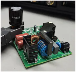
To outline how to apply LTspice to measure a capacitor’s ripple current, the DC2104A evaluation board was used. The demo board is an offline, boundary-conduction-mode (BCM) PFC boost converter based on the LT8312. It delivers a single 400-V, 150-W constant-voltage output, suiting it for applications that need a regulated input bus.

To start, short lead extensions must be added to the capacitor so that the current probe can be connected (Fig. 1). With the circuit running at input and output conditions where it will give the highest expected ripple current, the oscilloscope also must be adjusted so that the time window contains as much of an integral multiple of the waveform period as possible (Fig. 2).

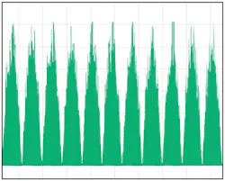
For ripple current waveform, the low-frequency components contribute more significantly to the capacitor’s internal heating than the high-frequency ones. For this reason, when performing an FFT, a time window that’s equal to an integer multiple of the lowest frequency component must be used; for this example, 120 Hz (100 Hz) was used.

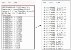
Next, export the captured ripple current waveform from the oscilloscope into a CSV file form. To ensure that LTspice can grasp the oscilloscope’s exported CSV data, the dataset must match the formatting illustrated in Figure 3. The process involves opening the CSV file in a text editor, removing the header row, and converting all comma delimiters to spaces.

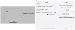
After editing the format of the data, create a new schematic in LTspice and copy the configuration shown in Figure 4 (left). This schematic consists of a piecewise linear (PWL) voltage source connected to a 1-Ω resistive load. Assign the edited CSV file to the PWL voltage source as illustrated in Figure 4 (right) and perform a transient simulation with a duration that matches the time span of the data captured from the oscilloscope.

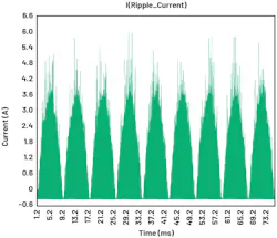
It’s important to use the latest version of LTspice before running the simulation. After all that, probe the current in the resistor to obtain the ripple current as shown in Figure 5.

Figuring Out Capacitor Ripple Current with FFT Analysis

For accurate FFT analysis, the input waveform must be continuous and repetitive. If the waveform displayed on the oscilloscope or LTspice has discontinuities at its edges, performing FFT on such data can lead to significant errors compared to the true value. To address this, a window function is applied to smooth out the discontinuities and make the waveform appear continuous.

However, in LTspice, the waveform can be zoomed to remove low-frequency discontinuities. It’s achieved by adjusting the time axis to display an integral multiple of the waveform period, which in this case is 120 Hz (100 Hz). To do this task, right-click the time axis and modify the leftmost, tick, and rightmost values accordingly. For example, in Figure 5, the value furthest to the left on the chart is 1.2 ms and the value furthest to the right is 76 ms.

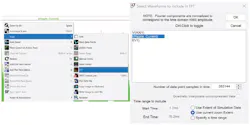
As shown in Figure 6 (left), with the waveform window active, navigate to “View” then “FFT” from the menu bar. Doing so generates the FFT to use the data from the current zoom extent selected and shown in Figure 6 (right).

Then right-click the y-axis to select linear representation and right-click the x-axis to edit the range from 10 Hz to 1 MHz to obtain the frequency domain of the ripple current (Fig. 7).

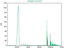
From the menu bar, choose File > Export Data as Text to generate a CSV file containing the FFT results. The data can be exported in either rectangular or polar format. The key requirement is to obtain the magnitude for each frequency (column D) using Equation 8 and then sort the values from highest to lowest (column F) as shown in Figure 8.

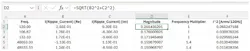
In this case, the I_ripple(Re) is the real component and I_ripple(Im) is the imaginary component of the exported current ripple data in rectangular form.

The frequency correction coefficient from the capacitor’s datasheet (column E) is required to calculate the ripple current for the base frequency. Use the ripple-current frequency obtained from the data (column A) to determine the capacitor frequency correction coefficient that should be used. Then, use Equation 6 to compute the effective ripple current of the capacitor.

In a BCM PFC converter, the switching frequency varies, so it’s important to sum as many frequency components as possible to closely approximate the actual ripple current.

However, in continuous-conduction-mode (CCM) PFC converters, where the switching frequency is fixed, the process can be simplified by selecting a few ripple current peaks at the switching frequency and its harmonics. The calculated effective ripple current for the first 1,000 highest peak points is 0.76A rms.

The estimated internal temperature rise (ΔT) can then be calculated using Equation 7, where capacitor‑rated specifications such as ripple current rating (I_O) and its corresponding internal temperature rise (ΔT_O) will come from the manufacturer’s data.

LTspice simulation offers an efficient and reliable way to estimate the effective ripple current in aluminum electrolytic capacitors in power-supply designs. Furthermore, the output provides a clear spectral component of each frequency. When combined with the datasheet-derived frequency correction coefficient, it allows for an accurate calculation of capacitor internal temperature rise and lifetime.