The Complete Guide to Troubleshooting and Fine-Tuning Digital Predistortion
Members can download this article in PDF format.
What you'll learn:
- What is digital predistortion?
- Architecture and operation of the DPD function.
- Configurations of, and setting up, the DPD function.
- How to deal with multiple issues that may arise with DPD.
- Using a compander for advanced tuning.
Digital predistortion (commonly known as DPD) is an algorithm widely used in wireless communication systems. DPD’s purpose is to suppress the spectral regrowth on the wideband signal that’s passed through the radio-frequency power amplifier (PA),1 thereby improving the PA’s overall efficiency.
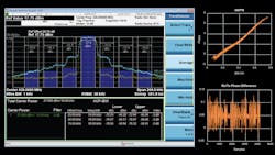
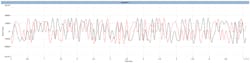
In general, PAs have nonlinear effects and inefficiency when dealing with high-power input signals. The nonlinear effect and the spectral interferences are caused by the spectral regrowth to the neighbor bands. Figure 1 shows spectrum regrowth before and after DPD correction using the TETRA1 standard on the ADRV9002 platform. The ADRV9002 offers an internal, programmable, and power-optimized DPD algorithm that can be customized to correct the nonlinear effect of the PA, thus improving the overall adjacent channel power ratios (ACPR).
Despite the desired benefits that DPD brings to communication systems, it’s often very difficult for an inexperienced person to start working with DPD, not to mention getting it set up properly. This is largely due to numerous factors that could contribute to errors and thus poor DPD performance. Even after hardware is set up properly, it may still be challenging to pinpoint the correct parameters to fine-tune DPD and obtain the optimal solution.
This article aims to help engineers who use the DPD option in the ADRV9002. It also includes some typical issues often encountered by a user, as well as providing some general strategies on fine-tuning a DPD model with the available parameters to obtain optimal DPD performance.
The device also includes a MATLAB tool to help users analyze DPD. This should help eliminate many common mistakes and provide some insights on the internal DPD operations. What’s presented here will help users get started with DPD and provide useful information on both theoretical concepts and resolving practical issues.
The ADRV9002 offers up to 20-MHz signal bandwidth when enabling the DPD option. This is due to the receiving bandwidth being limited to 100 MHz. Typically, DPD will operate with a receiving bandwidth 5X the transmitter bandwidth, so that the third and fifth intermodulation signals can be seen and corrected.
The highest PA peak power signal supported by the ADRV9002 is around the 1-dB (commonly known as P-1dB) compression region. This metric indicates the severity of PA compression. If the PA is compressed beyond the P-1dB point, it’s not guaranteed that DPD will work properly. However, this isn’t a strict requirement. As we have seen in many cases, DPD works over the P-1dB point and still provides very good ACPR. It’s going to be a case-by-case investigation, though.
In general, if the compression is too severe, DPD can potentially run into instability and crash issues. We will discuss more about the compression region in later sections, including how to observe the current PA compression status using the MATLAB tool.
More details on DPD can be found in Analog Devices’ UG-1828 User Guide, in the “Digital Predistortion” chapter.
Architecture
There are two basic approaches to perform the DPD function. The first is called an indirect DPD, where a signal is captured before and after the PA. This differs from the direct DPD approach in which a signal is taken before the DPD block and after the PA. The advantages and disadvantages of each are beyond the scope of this article.
Indirect DPD looks at the signal before and after the PA to learn its nonlinear behavior and does the reverse on the DPD block. Direct DPD looks at the signal before DPD and after the PA and eliminates the error between the two by applying predistortion on the DPD block. Users should know that the ADRV9002 uses the indirect approach and the implications that are associated with it. It’s also important to know when using the MATLAB tool, capture data also refers to the indirect approach.
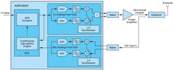
Figure 2 shows a high-level DPD operation block diagram for the ADRV9002. Input signal u(n) goes into the DPD block. DPD will predistort the signal and generate x(n). Here, we call this transmit capture, although it’s really the predistorted version of the transmit signal.
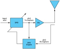
The signal then goes through the PA to become y(n), which eventually gets sent out into the air. We call y(n) the receive capture, although it’s really the transmit signal after the PA. y(n) then feeds back to the receiver port, used as an observation receiver. Essentially, the DPD engine will take captures of x(n) and y(n), then generate the coefficients, which will be applied in the next iteration of DPD.
Mode of Operation
ADRV9002 supports both TDD and FDD operations on DPD. In TDD mode, DPD is updated for every transmit frame. This means the receiver will act as an observation path during the transmit frame. In FDD, since the transmitter and receiver are both running at the same time, a dedicated receiver channel is needed. ADRV9002 has 2T2R, which can support DPD in 2T2R/1T1R TDD and 1T1R FDD modes.
DPD Model
Structure
The following equations show the DPD model implemented in the transmit path:
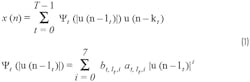
where:
- u(n) is the input signal to DPD x(n) is the output signal of DPD.
- T is the total number of taps of the DPD model.
- ψt is the polynomial function to implement the lookup table (LUT) for tap t lt is the amplitude delay.
- kt is the data delay.
- at,lt,i is the coefficient calculated by the DPD engine.
- bt,lt,I is the switch to enable or disable the term.
- i is the index and power of the polynomial term.
Users can configure the number of polynomial terms for each tap. ADRV9002 provides three memory term taps and one cross term tap, each with an order from 0 to 7.
Model Selection
Users may select a default model option provided by ADRV9002 (Fig. 3), which should work for most common cases. Alternatively, users can choose their own model by enabling and disabling terms. The first three taps (0 to 2) indicate the memory terms, where Tap 1 is the center tap. Tap 3 is the cross term tap.
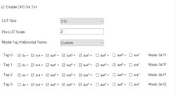
Note Tap 3 (or the cross term tap) should not have the zeroth-order term enabled, to differentiate from the memory term taps.
- LUT size: Users can set the LUT size. The ADRV9002 provides two options, 256 and 512. With the 512 size, users will have a better quantization noise level, and thus better ACPR, as a larger size will generally provide a better resolution of the signal. For narrowband applications, we recommend using 512 as the default option. 256 could be used for wideband as the noise level isn’t as stringent, and the computation and power can be improved.
- Pre-LUT scale: Users can set the pre-LUT scaler to scale the input data to fit better on the compander. The compander takes the signal from the transmitter and compresses it to fit in the 8-bit LUT address. Depending on their input signal level, users can adjust this value to optimize the LUT utilization. The values can be set in range (0, 4) with a step of 0.25. There’s more on the compander in the last section of this article.
Configurations
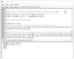
To perform DPD, users will have to enable an external loopback path on the PA and then set the feedback power to make sure it’s not out of range (Fig. 4). Note it’s the peak power, not the average power. Power that is too strong or too weak will impact DPD performance. Users also need to set the external path delay, which can be obtained using External_Delay_Measurement.py. This script can be found in the ADRV9002 evaluation software installation path under the IronPython folder.
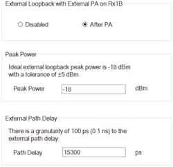
The external delay only needs to be set for high sample-rate profiles (for example, LTE 10 MHz). For low sample-rate profiles (TETRA1 25 kHz), the user can set it to 0. Later in this article, we will use the software tool to observe the capture data to see the external delay effect.
Additional Settings
Users can configure the number of samples (Fig. 5). By default, users can set 4096 samples. It’s recommended to use default values.
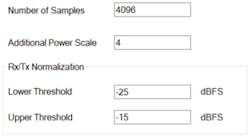
In most cases, the default 4096 samples will provide optimal solutions for DPD.
- Additional Power Scale: This is a more advanced parameter. For the most part, it’s recommended to use the default value of 4 for the ADRV9002. This parameter has to do with the internal correlation matrix. From our experiment, the default value gives the best performance for the existing waveforms and PAs we tested. In rare cases, where input-signal amplitude is extremely small or large, users can try to adjust this value to smaller and larger values so the correlation matrix maintains a proper condition number and therefore more stable solution.
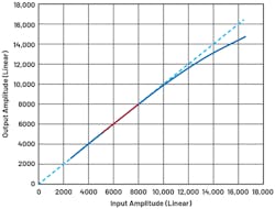
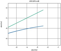
- Rx/Tx Normalization: Users should set the receiver/transmitter normalization to the region where the data is linear. In Figure 6, the linear region is shown in red. In this region, the power of data hasn’t reached the compression region and is high enough for gain calculation. Once the region is selected, DPD can make an estimate on the gain of the transmitter and receiver, and then proceed with further processing on the algorithm. For most cases, –25 to –15 dBFS should accommodate most standard PAs. However, users should still pay attention as special PAs could have very different shapes of AM/AM curves, in which case a proper modification will be needed. This will be described in more detail in later sections of this article.
Setup
Hardware Setup
A typical setup is shown in Figure 7. A low-pass filter is needed before the signal goes into the PA, to prevent LO signal harmonics. In certain cases, where internal LO phase-noise performance doesn’t satisfy the application, external LO may be needed.
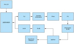
In such a case, the external LO source needs to be synchronized with DEV_ CLK. This is typically needed for narrowband DPD, where the close-band noise requirement is more stringent.
It’s generally recommended to have a variable attenuator before the PA to prevent potential damage to the PA. The feedback signal should have the proper attenuation to have peak power set as discussed in the previous section.
Software Setup
IronPython
Download the IronPython library to execute the IronPython code on the GUI.
Here, users can run dpd_capture.py in the IronPython window in the GUI (Fig. 8), provided along with the MATLAB tool to get capture data for the transmitter and receiver. The DPD sample rate also is included as part of the captured file.
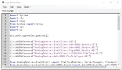
Note this script should be run either in a primed or calibrated state.
MATLAB Tool
The MATLAB tool analyzes the captured data from dpd_capture.py. This tool will help check signal integrity, signal alignment, PA compression level, and, at last, the fine-tuning of DPD.
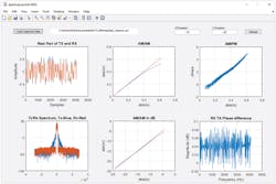
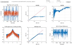
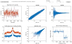
The MATLAB tool requires MATLAB Runtime. A first-time install will take some time to download. Once installed, users can load the data that’s captured by the IronPython script, and then observe the plots (Fig. 9).
Users also can set the high/low threshold on the normalization of the data and hit Reload to see the changes.
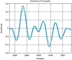
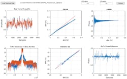
First, we have the normalized transmitter and receiver data plotted in the time domain. Users can zoom in to observe the status of the alignment of the transmitter and receiver. We only show the real part of the data, but users can easily plot the imaginary part as well. Normally, real and imaginary parts should both be either aligned or unaligned.
Then we have the transmitter and receiver spectra—the blue is transmitter and red is receiver. Note this is indirect DPD—the transmitter data will be the predistorted data, not the transmitter datapath over the SSI port.
Next, we have two AM/AM curves, both in linear and dB scales. These are important metrics on DPD performance and PA compression status.
The AM/PM curve and receiver/transmitter phase difference also are provided.
In addition, we have the high and low threshold numbers. These numbers should match what’s set in the ADRV9002 TES evaluation software.
Since we’ve provided APIs to capture data, users can develop their own plots and analysis models if needed. The tool provides some of the common checks for analyzing DPD. The APIs are:
- adi_ADRV9002_dpd_CaptureData_Read, which is the read DPD captured data and must be run in a calibrated or primed state.
- adi_ADRV9002_DpdCfg_t → dpdSamplingRate_Hz, which is the DPD sample rate, read-only parameter.
Typical Issues
DPD can be affected by many different factors. Therefore, it’s worthwhile to make sure all of the potential issues listed are considered and examined by the user. Before considering all issues, users should make sure hardware is connected correctly.
Transmit Data Overload
Figure 10 shows a high-level block diagram of DPD implementation by ADRV9002. Transmitter data coming from the interface can overload the DAC. If the DAC is overloaded, the RF signal of the transmitter will be distorted even before involvement of the PA. Therefore, it’s critical to make sure transmitter data doesn’t overload the DAC.
To see if the transmitter DAC is overloading, users can just observe it from the GUI. Figure 11 shows a TETRA1 25-kHz waveform. The peak is still far away from the digital full scale. For the ADRV9002, it’s recommended to be at least a few dB from full scale, to avoid potential overload of the DAC.
It’s difficult to quantify how much users should back off—this is because DPD will try to perform predistortion, and the predistorted signal will be “peak expanded,” potentially overloading the DAC. This depends on how DPD is reacting to a particular PA—generally, the more compressed the PA, the more room it needs for peak expansion.
Receiver Data Overload
Another common error is the receiver data overloading the feedback ADC (Fig. 12). This is caused by not having enough attenuation going back to the receiver port. The effect, as you can observe from the debugging tool, is that receiver data is clipped, Because of this, the transmitter and receiver can’t effectively align, causing DPD to have a calculation error. DPD typically will behave extremely poorly, resulting in increased noise on the whole spectrum.
Receiver Data Underload
Compared to receiver overload, this issue can often be overlooked. It’s caused by not properly setting the feedback attenuation. A user may put too much attenuation to the feedback path, which makes receiver data too small. By default, –18 dBm peak is recommended for the ADRV9002 because it will bring the data from analog to digital to a good known power level for DPD. However, users can tune this number to fit their needs.
Users should know that the DPD feedback receiver doesn’t use the same attenuator that regular receivers use, and it has a much higher step size. The level of attenuation is adjusted by the peak power level set by the user. The lowest power level is –23 dBm (with 0 attenuation)—beyond that, users will run into low power levels, which will impact DPD performance.
As a rule of thumb, users should make sure the feedback power is always measured and set correctly. Oftentimes, users tend to try different power levels and forget to set the feedback power properly, which causes this issue.
TDD vs. FDD
DPD in TDD mode must be run in the automated state machine. When evaluating with TES, in the manual TDD mode, users can still enable DPD. However, performance will be poor because DPD will only operate frame-based.
In manual TDD mode, the length of a frame will be determined by the transmit/receive enable signal toggle. In other words, each play and stop is a frame. However, in the time it takes for a human being to toggle, the PA has already turned to a different state in terms of temperature. Therefore, it’s impossible to maintain the DPD state without using the automated TDD mode where transmit enable signals can be frequently toggled. In FDD mode, though, DPD should perform normally.
For example, a user may want to use TETRA1, which follows a TDD-like frame scheme (it’s actually TDM-FDD). Therefore, directly selecting TDD mode and manually checking DPD will not be desired, and DPD tends to perform poorly. Instead, users can either use the “Custom FDD” profile and pick the same sample rate and bandwidth as TETRA1, or users can set TETRA1 TDD frame timing and use automated TDD mode. Both methods typically offer much better performance than manual TDD.
Transmitter/Receiver Unaligned
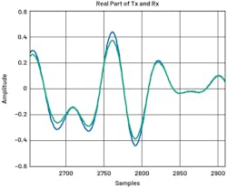
ADRV9002 will try to time-align transmitter and receiver data. When data is captured by a user, it’s expected to be aligned (Fig. 13). The delay measurement is done in the initial calibration time. However, for high sample-rate profiles, more precise subsample alignment needs to be done separately.
DPD is an adaptive algorithm that requires taking the error of the two entities, aka the transmitter and receiver. Before taking the error of the transmitter and the receiver, the two signals need to be properly aligned—especially if a high sample-rate profile is used (for example, LTE10) (Fig. 14). The alignment is critical because the intervals between samples are small. Therefore, users will need to run the script External_Delay_Measurement.py to extract the external path delay (Fig. 15). This number can be entered under Board Configuration → Path Delay.
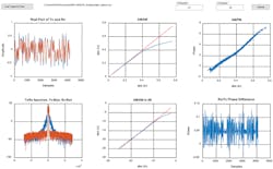
The effect of not having transmitter and receiver data aligned is that users will observe a much noisier AM/AM curve.
After setting the path delay number, we can observe the AM/AM and AM/PM curves to be much cleaner and less noisy (Fig. 16). Phase difference is also much smaller (Fig. 17).
PA Overload
Each PA has its own specification in terms of how much compression it can handle. Although the P-1dB data is typically given in the datasheets, from a practical standpoint, it’s still recommended to take precise measurement on the DPD to make sure that the compression point is at P-1dB (Fig. 18). The DPD software provides the user the ability to look at the AM/AM curve based on the captured data to observe how close the compression point is compared to P-1dB.
If, however, a signal is beyond P-1dB, then this will potentially cause DPD to be unstable or even break, having the spectrum jump to a very high level and never come back down. In Figure 19, compression is way beyond the 1-dB region on the peaks, and the shape of the curve also starts to become flatter. This is a sign that the PA is overdriven; to increase more power on the output, input will be pushed a lot more to support the output power level. At this point, in case the user decides to continue to increase the input power, the DPD performance will decrease.
General Strategy Model Picking and Tuning
The idea of indirect DPD is to have data captured before and after the PA, while the DPD engine will try to mimic the opposite effect of the PA. The LUTs are used to apply this effect using the coefficients, and the model is polynomial-based. This means DPD is more like a curve-fitting problem, and users will try to use the terms to “curve fit” the nonlinearity effect.
The difference is the curve-fitting problem fits a single curve, while DPD also must account for the memory effect. ADRV9002 has three memory taps and one cross tap for modeling DPD LUTs.
Figure 20 shows the three memory taps and the one cross tap provided by ADRV9002. The general strategy is similar to a curve-fitting problem. Users can start with some baseline and add and remove terms. In general, a center tap must exist (Tap 1).
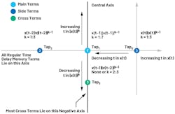
Users can add and remove terms one by one to test the effect of DPD. Then they can add two more memory taps (taps 0 and 2) to add in the effect of memory-effect correction. Since the ADRV9002 has two side taps, these taps should be the same—that is, symmetrical. Adding and removing terms should also be done by a one-by-one approach. Lastly users can experiment with cross term. Cross terms complete the curve-fitting problem from a mathematics point of view, thus providing better performance from DPD.
Note users should not skip terms by leaving them blank, as this will cause DPD to have undesired behavior. Moreover, users should not set the zeroth term on the cross term tap, as this isn’t valid from a mathematics point of view as well.
Advanced Tuning
Compander and Pre-LUT Scaler
In a previous section, we mentioned the compander. When first reading the user’s guide, this concept may create some confusion on what it means or what to choose (256 or 512). The purpose of the compander is to compress the input data and fit it in the lookup table (LUT).
The general shape of the compander is a square root, where you have I/Q data coming in (Fig. 21). Before we put them in the LUTs, the equation (√(i(n)2 +q(n)2) will be used to get the signal magnitude from previous equations. However, since square root is an expensive operation in terms of speed, and we need to map them into a LUT (8 bits or 9 bits), we turn to the compander.
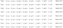
Figure 22 is the ideal square-root curve. The actual implementation will not be shown here, but in short, it’s going to be an estimation of the square-root curve.
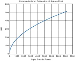
Once we understand how data is fit into the LUTs, we can start tuning data more intelligently. ADRV9002 has the option of choosing 8 bits (256) or 9 bits (512) for the LUT size. A bigger LUT means doubling the address locations for data. This means a finer resolution of the data and, in general, a better quantization noise level.
For narrowband applications, since the noise is so important, we recommend always using the 512 option. And for wideband applications, since noise level isn’t so crucial, either option can be used. But if the 512 option is used, slightly more power will be consumed and computation will be slower.
Histogram and CFR
We briefly mentioned pre-scale in DPD configuration. This parameter is used to provide a boost of the input data to LUTs. This boost is needed because in some cases, the data isn’t utilized properly by DPD. For a PA compression problem like this, it’s the high-amplitude samples that really get compressed and cause problems. Therefore, we must not treat all samples equally; instead, we want to focus our attention on the high amplitude samples.
Take a look at the TETRA1 standard waveform histogram (Figs. 23 and 24). We can observe that most values occur on medium- to high-amplitude regions. The reason is because the TETRA1 standard uses a D-QPSK modulation scheme, and the result is the signal will have constant envelope. The peak power doesn’t differentiate too much from the average power.
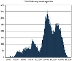
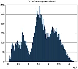
This is desired for DPD. As mentioned previously, DPD will catch more high-amplitude samples and therefore better characterize the behavior of the PA.
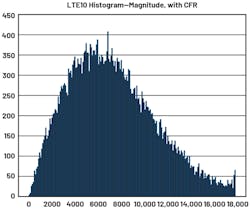
Now we look at the LTE10 standard in a similar way (Fig. 25). LTE uses an OFDM modulation scheme, which combines hundreds and thousands of subcarriers together. Here we have the magnitude and power again for LTE10. We can easily observe the difference in contrast to TETRA1—the peaks are very far away from the main average.
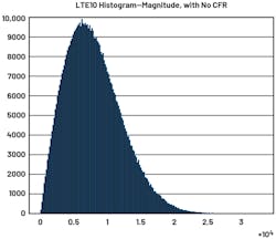
In the power histogram (Fig. 26), if we zoom in on the far end, we can observe that very high peaks are still occurring, but with very low probability. This is very undesirable for DPD. There are two reasons.
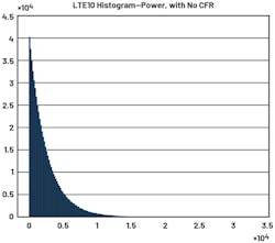
First, the low probability count of high peaks (high-amplitude signals) will make the PA extremely inefficient (Fig. 27). For example, LTE PAPR is about 11 dB. That’s a big difference. To avoid damaging the PA, the input level will need to back off by a very big margin. Therefore, the PA isn’t utilizing the majority of its gain ability to boost power.
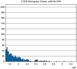
Second is the high peaks also are wasting the utilization of the LUTs. Due to these high peaks, LUTs will allocate a lot of resources for them and only a small portion of the LUTs are allocated for most of the data. This will degrade the DPD performance.
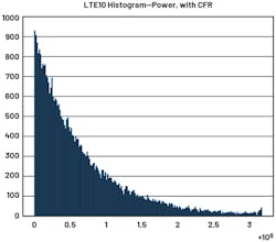
Crest factor reduction (CFR) is a technique that moves the signal peaks down to a level that’s more acceptable. This is typically used in OFDM-type signals. ADRV9002 doesn’t include on-chip CFR, so this function needs to be implemented externally. In the ADRV9002 TES evaluation software, we also include the CFR version of the LTE waveforms for this purpose.
CFR_sample_ rate_15p36M_bw_10M.csv is shown in Figure 28. We can observe at high power, the signal is being peak-limited to a certain level (tilt at the end), due to CFR. This effectively pushes the PAPR to about 6.7 dB, which is almost a 5-dB difference.
The operation of CFR will “hurt” the data, in the sense that error vector magnitude (EVM) will degrade. However, compared to the whole waveform, the high-level amplitude peaks have very small probability of occurrence and the benefits are tremendous (Fig. 29).
Reference
1. D.R. Morgan, Z. Ma, J. Kim, M. G. Zierdt, and J. Pastalan. “A Generalized Memory Polynomial Model for Digital Predistortion of RF Power Amplifiers.” IEEE Transactions on Signal Processing, Vol. 54, No. 10, October 2006.
About the Author
Wangning Ge
Product Applications Engineer, Analog Devices Inc.
Wangning Ge was a product applications engineer based in Somerset, New Jersey. He joined Analog Devices in 2019. Previously, he worked as a software engineer at Nokia (formerly Alcatel-Lucent). Wangning has experience in DPD algorithm design and base-station radio applications. He was responsible for the ADRV9001 family of transceiver products.
Comment About the Article
To join the conversation, and become an exclusive member of Electronic Design, create an account today!

Leaders relevant to this article: