Selecting Minimum/Maximum Noise Frequencies for Transient Noise Simulation

Controlling noise is critical when it comes to designing advanced analog and radio-frequency (RF) circuits. In the digital world, designers tend to tackle noise by adding ground planes, shortening high-speed traces, and placing decoupling capacitors close to IC power pins.

However, high-performance analog designs have significantly tighter noise margins. The most important performance metrics in these scenarios — such as signal-to-noise ratio (SNR), bit error rate (BER), phase noise, and timing jitter — rise or fall with noise.

The challenge is that a significant amount of noise is baked directly into the semiconductor devices themselves and, therefore, can’t be avoided. As a result, device noise ultimately sets the fundamental limits of the circuit’s functionality.

The problem is particularly acute in analog circuits with noise-sensitive architectures, including those based on the most advanced CMOS process nodes, where falling supply voltages and rising operating frequencies leave little headroom. The complex building blocks in these designs, including analog-to-digital converters (ADCs), phase-locked loops (PLLs), transmit and receive (Tx/Rx) chains, and high-speed SerDes, all operate close to these limits. Consequently, they’re all susceptible to device noise, which is often highly transient.

Transient noise analysis plays a significant role in analog design by simulating a circuit’s response to random device noise. Unlike a conventional transient circuit simulation, a transient noise simulation models the inherent noise of its circuit elements. More specifically, a transient noise simulation includes thermal noise for non-ideal resistors and MOS/bipolar device noise sources (1/f noise, MOS gate thermal noise, and bipolar shot noise).

When performing a transient noise simulation, values must be specified for the minimum and maximum frequency of the noise sources and simulation accuracy. As outlined in Reference 1, the accuracy of a transient noise simulation is highly dependent on these parameters.

The lowest frequency the simulation can capture is governed by the simulation end time TSTOP. Since a full period of frequency components whose period is greater than TSTOP isn’t included in the simulation data, the magnitude of these frequency components can’t be accurately determined. Thus, a reasonable choice for the minimum frequency of noise sources is 1/TSTOP Hz.

To understand the need for a maximum noise frequency limit in a transient noise simulation, consider the impact of a resistor’s thermal noise on a circuit simulator. Without a limit to the maximum noise frequency, the time increment (i.e., timestep) that must be taken by a circuit simulator approaches zero, as very small timesteps are necessary to include high frequencies of the noise. Therefore, one must set a maximum noise frequency to limit the minimum simulation timestep to a reasonable value.

Oftentimes, it’s not obvious how high the maximum noise frequency should be set for linear and nonlinear circuits. Choosing a large value for the maximum noise frequency forces the simulator to use small timesteps to create the high frequency noise. In turn, it prolongs the simulation time and increases the size of the simulator output file.

Conversely, choosing too low of a value for the maximum noise frequency may not provide an accurate estimate of circuit noise. That’s because any noise components existing above the specified maximum noise frequency will not be included.

Striking the right balance will produce an accurate estimate of noise metrics from the simulation results.

Transient Noise Simulation of Linear vs. Nonlinear Circuits

If the circuit being examined is linear — for instance, an amplifier operating in its linear region — the transient noise frequencies will mirror the noise source frequencies shaped by the gain and bandwidth of the circuit.

There’s no frequency translation of noise frequencies. Consequently, increasing the maximum source noise frequency has no impact on low frequency noise. Thus, an appropriate maximum noise frequency is determined by the bandwidth of the desired noise measurement. If the maximum transient noise bandwidth exceeds the bandwidth of the noise measurement, it will not impact the noise measurement.

If the circuit is nonlinear, then the transient noise sources can undergo frequency translation and introduce components of noise at frequencies dependent on the frequency or frequencies of the input stimuli and the frequency of the noise sources. Aliasing of noise source frequencies from high frequencies to low frequencies may occur depending on the source noise bandwidth relative to the stimulus frequency or frequencies.

The case of the nonlinear circuit serves as the motivation for quantifying the spectral components of input stimuli. The reason is that only significant frequency components of the input stimuli will contribute to transient noise frequency translation and potential aliasing. If you have an estimate of the spectral bandwidth of the input stimuli, a value for the maximum source noise bandwidth may be chosen to produce an accurate estimate of transient noise.

Impact of Amplitude-Modulated Square Waves with Random Noise

When a periodic square wave is amplitude-modulated by a modulating signal, the modulating signal’s spectrum is frequency-translated to each of its harmonics and a possible DC term of the square wave.

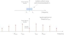
Figure 1 illustrates the frequency spectrum for a noise spectrum with a finite bandwidth (fn) and a square wave of fundamental frequency (fpulse) with a possible DC term, and all of the harmonics of fpulse.

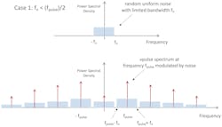
When the noise spectrum amplitude modulates the square wave, the amplitude-modulated spectrum will appear similar to either Figure 2 or Figure 3. If the noise bandwidth (fn) is less than 50% of the fpulse, the noise spectrum is centered about each harmonic and doesn’t extend to any adjacent harmonic (Fig. 2).

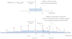
However, if the bandwidth of the noise exceeds 50% of fpulse, then Figure 3 depicts the regions of overlap where the noise impacts not only the harmonic about which it’s centered, but adjacent harmonics.

This example illustrates the impact of the maximum noise frequency in a transient noise simulation. Since the noise sources will amplitude-modulate the input stimuli, the noise of the amplitude-modulated spectrum will depend on the bandwidth of the noise relative to the input stimuli. Noise bandwidths that exceed 50% of the input’s frequency will alias to lower frequencies and increase low-frequency noise.

If the transient noise bandwidth encompasses all significant harmonics of the input stimuli, the results of the transient noise simulation will provide an accurate estimate of aliased low-frequency noise. However, if the noise bandwidth is chosen to be less than the number of significant input signal harmonics, the simulation results may not accurately estimate low-frequency noise.

Encapsulating Device Noise with Simulations and Example Waveforms

To explore the magnitude of low-frequency noise as a function of the input noise bandwidth, six example 100-MHz square waveforms were amplitude-modulated by random uniform noise with a modulation index of 0.25 using the program outlined in Reference 2.

The relative harmonic powers for each of the six waveforms are shown in Figure 4. Using a metric of 20 dB to define the spectral bandwidth, the bandwidth of each waveform is shown by the border between the red and white shaded regions.

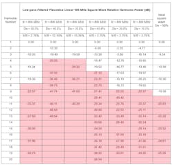
What stands out is the very significant even harmonic power as the duty-cycle distortion increases. In essence, the number of significant harmonics when it comes to a square wave with a fair amount of duty-cycle distortion is twice the number when examining a waveform with very little.

The two waveforms with duty cycles of 20% and 70% are also modulated using Gaussian random noise in lieu of uniform random noise, with a modulation index of 0.10 to form a total of eight simulated amplitude-modulated waves.

The bandwidth of the uniform or Gaussian noise was varied from 10 MHz to 8 GHz, and the power spectral density of each amplitude-modulated waveform was computed. By integrating the power spectral density results over 90 MHz (excluding DC), the low-frequency rms noise was computed to quantify the relationship between the rms noise and the input noise bandwidth.

Since the amplitude modulation produces phase modulation of the waveforms, the time interval error (TIE) of each amplitude-modulated waveform, and its phase noise, was also computed. The rms jitter of each was determined in the temporal and frequency domains and plotted against the input noise bandwidth.

The power spectral densities of one of the 100-MHz square waves, when it’s amplitude-modulated with uniform noise of bandwidths 30 MHz and 300 MHz, are depicted in Figure 5. The two input noise bandwidths of 30 MHz and 300 MHz represent examples of the tutorial cases shown in Figures 2 and 3, where the noise bandwidth is less than and greater than half the square-wave fundamental frequency, respectively.

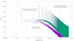
Figure 5 illustrates the added low-frequency noise due to the aliasing when compared to the 100-MHz square-wave spectrum modulated with uniform noise whose bandwidth is 30 MHz.

Noise in the Circuit: How Transient Noise Bandwidth Impacts Voltage Noise

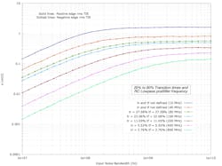
The next step is to examine the simulation results. Figure 6 provides the integrated voltage noise for each of the eight amplitude-modulated square waves. The integrated value approaches a different asymptote as the noise bandwidth is increased. In addition, the noise bandwidth will vary when the value reaches its asymptotic value.

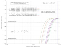
The dotted lines in Figure 6 are curve fits to each data set using the equation outlined in the same figure, with coefficients C₀, C₁, and C₂.

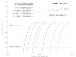
Normalizing the curve fits to their maximum asymptotic value yields the expanded x- and y-axis view in Figure 7.

The curve-fit coefficients and the noise bandwidth frequencies for each waveform that correspond to 95% and 99% of its asymptotic rms noise voltages are provided in Figure 8 with the −20 dB threshold spectral bandwidths for each waveform from Figure 4.

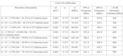
To estimate the maximum noise frequency for the simulation, it makes sense to compare the −20 dB harmonic threshold of each waveform to the frequency corresponding to 99% of its asymptotic rms noise. In that case, the maximum transient noise bandwidth should be set at or above the frequency of the transient signal beyond which its harmonic powers are less than 20 dB from its fundamental harmonic power.

Choosing a smaller maximum transient noise bandwidth will produce more than a 1% error in the rms voltage.

How Phase Noise Happens and Its Relation to Transient Noise Bandwidth

The last section focused on the relationship between transient noise bandwidth and the rms voltage noise, ranging from low frequencies through to the frequency of the fundamental harmonic of an amplitude-modulated square wave.

However, amplitude modulation will also produce phase noise. Phase noise is introduced when the threshold crossings are modulated by changes in amplitude. The amplitude-to-phase-noise transfer function is frequency-dependent. At frequencies higher than the inverse of the signal or systems-dominant time constant, the magnitude of the transfer function decreases.

So, how does the value chosen for the maximum transient noise bandwidth relate to the accuracy of the phase noise estimate it produces? To answer this question, a set of simulations follow that provide insight into the appropriate maximum transient noise bandwidth for a transient noise simulation to accurately estimate phase noise.

To quantify the transfer function relating amplitude modulation to phase modulation, a 133-MHz sinusoid was amplitude-modulated with sinusoids between 1 MHz and 10 GHz using a modulation index of 0.10.

The amplitude-modulated sinusoid was followed by a single-pole low-pass filter whose cutoff frequency was set to 100 MHz, 250 MHz, and 500 MHz. The low-pass filter represents the dominant time constant of the signal. The TIE in unit intervals (UI) was measured for each modulated waveform, and its rms value is depicted as a function of the modulation frequency for each low-pass filter seen in Figure 9.

The transfer functions of amplitude to phase modulation increase with modulation frequency, which will continue to rise until it exceeds the low-pass filter cutoff frequency representing the signal's dominant pole. Since the amplitude modulation consists of a single frequency, the transfer function becomes less as the modulation frequency increases beyond the signal's dominant pole frequency.

If the amplitude modulation consisted of many frequencies, the slope of the transfer function would approach zero. That’s because higher modulation frequencies don’t add to the total phase modulation.

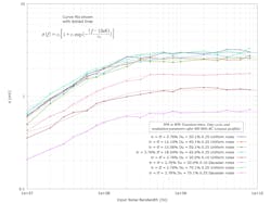
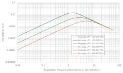
Extending the amplitude modulation from a single sinewave to uniform noise, the rms phase jitter was computed for a set of 100-MHz square waves amplitude-modulated by uniform random noise. The bandwidth of the noise was varied between 10 MHz and 10 GHz. An RC low-pass filter was varied from 10 MHz to 800 MHz to reflect the signal or system’s dominant pole.

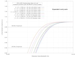
The rms jitter can be found in Figure 10 with an expanded and normalized view of its curve fits in Figure 11. The rms jitter exhibits an asymptotic behavior with modulation bandwidth whose corner frequency is related to the dominant pole of the square wave or system. Looking closely at Figure 11 reveals that when the noise bandwidth exceeds about 10X the signal or system’s dominant pole frequency, the rms jitter is less than 1% from its asymptotic value.

Referring to the single sinusoid modulation results in Figure 9, the factor of 10 from the dominant pole represents the frequency where it will attenuate the modulating noise by 20 dB. At modulation frequencies higher than this, the input noise no longer significantly contributes to the phase noise. The upshot is that to achieve an accurate estimate of the rms phase jitter in a transient noise simulation, it should be set to 10X the frequency of the dominant pole of the signal or system being examined.

To further validate the hypothesis, the rms jitter for each of the eight 100-MHz amplitude-modulated square waves was computed for input noise bandwidths between 10 MHz and 10 GHz. Although the duty cycles, transition times, type of noise, and modulation indices differ, each of these waveforms has a dominant pole of 800 MHz.

The normalized curve fits for the integrated phase noise for each waveform as a function of the input noise bandwidth is provided in Figure 12. The frequency at which the rms jitter reaches its asymptotic value varies. However, for an input noise bandwidth of 8 GHz (10X the 800-MHz dominant pole frequency), the rms jitter for all cases is within 1% of its asymptotic value.

Pole Position: Pinpointing the Dominant Pole of a Signal or System

To reiterate, a very good estimate of a signal’s rms jitter in a transient noise simulation is achieved when the maximum transient noise bandwidth is 10X the dominant pole of the signal or system. But how do you determine the dominant pole frequency in the first place?

If the transition time of a waveform or output signal of a system is dominant pole limited and measured between two thresholds, the −3 dB bandwidth for the corner frequency of the effective low-pass filter that will produce the same transition time may be determined using Equation 1.

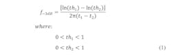
For example, if one measures the maximum 20% to 80% transition time as 1 ns, Equation 2 indicates the −3 dB bandwidth is 220.6 MHz. Therefore, to estimate the phase noise for this signal in a transient noise simulation that will provide an rms jitter accuracy of less than 1%, the maximum noise bandwidth should be set to at least 10 × 220.6 MHz, equaling approximately 2.2 GHz.

By examining the slope of the minimum transition time of the signal, some insight into the nature of the limiting mechanism is possible. If it’s dominant pole limited, the slope of the transition will be exponential in nature. If the minimum transition is limited by a different mechanism (such as current limited), its slope may appear linear or constant. In this case, a Fourier analysis of the signal may be helpful to estimate its dominant pole frequency.

Figure 13 compares the power spectral densities of two 100-MHz square waves with identical 20% to 80% transition times of 12.1%. However, one waveform has piecewise linear 20% transition times and is followed by an 800-MHz low-pass filter; the other waveform has piecewise linear 0.10% transition times and is followed by a 182.3-MHz low-pass filter. The transition times of the former waveform aren’t dominant pole limited, whereas the latter are as result of its 182.3-MHz low-pass filter.

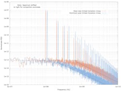
Inspecting the noise floor of each waveform provides an estimate of the system’s dominant pole. The dotted asymptotes shown in Figure 13 provide a good estimate of the dominant system poles of about 800 MHz and 180 MHz for the former and latter waveforms.

Summary and Recommendations for Transient Noise Simulations

To estimate a value for the maximum transient noise bandwidth for a transient noise simulation, a set of the 100-MHz waveforms was amplitude-modulated by uniform and Gaussian random noise, whose bandwidth was varied from 10 MHz to 8 GHz. In effect, this represents the use of a noise bandwidth of between 10 MHz and 8 GHz in a transient noise simulation.

For each waveform, the relationship between rms voltage noise and input noise bandwidth suggests that beyond a specific input noise bandwidth, the rms noise approaches an asymptotic value.

From this data, the minimum input noise bandwidth for the rms noise to be within 1% of its asymptotic value is found to correlate well with the frequency at which the square wave’s harmonics are 20 dB lower than its fundamental power.

Since the amplitude modulation can induce phase modulation, the study also analyzed the minimum noise bandwidth to accurately estimate the jitter due to the conversion of amplitude noise to phase noise. Unlike the rms voltage noise results, the minimum input noise bandwidth at which the integrated phase noise approaches its asymptotic value correlates most closely with the bandwidth of the dominant signal or system pole.

In conclusion, to ensure an accurate estimate of the voltage noise in a transient noise simulation, the maximum transient noise bandwidth should be set to the frequency at which the harmonic power of the signal of interest remains below 20 dB from its fundamental harmonic.

To accurately estimate the phase noise in a transient noise simulation, the maximum transient noise bandwidth should be 10X the frequency of the dominant signal or system pole. For a deeper dive, Reference 3 offers an expanded version of this study.

References

1. Guyton, Scott. “Full Spectrum Transient Noise: A must have sign-off analysis for silicon success,” January 29, 2025.

2. Logan, S. M. “Description, Installation, and Use of vpulse: A Program to Create a Sampled Piecewise Linear Periodic Square Wave,” March 18, 2025, v1.10.

3. Logan, S. M. “Selecting the Minimum and Maximum Noise Frequencies in a Transient Noise Simulation to Produce Accurate Noise Measurements,” February 21, 2025, v1.0.